


(C) 2012 Dirk S. Schmeller. This is an open access article distributed under the terms of the Creative Commons Attribution License 3.0 (CC-BY), which permits unrestricted use, distribution, and reproduction in any medium, provided the original author and source are credited.
For reference, use of the paginated PDF or printed version of this article is recommended.
Conservation of habitats is a major approach in the implementation of biodiversity conservation strategies. Because of limited resources and competing interests not all habitats can be conserved to the same extent and a prioritization is needed. One criterion for prioritization is the responsibility countries have for the protection of a particular habitat type. National responsibility reflects the effects the loss of a particular habitat type within the focal region (usually a country) has on the global persistence of that habitat type. Whereas the concept has been used already successfully for species, it has not yet been developed for habitats. Here we present such a method that is derived from similar approaches for species. We further investigated the usability of different biogeographic and environmental maps in our determination of national responsibilities for habitats. For Europe, several different maps exist, including (1) the Indicative European Map of Biogeographic Regions, (2) Udvardy’s biogeographic provinces, (3) WWF ecoregions, and (4) the environmental zones of
Conservation tools, environmental zones, habitat conservation, national responsibility, prioritization, scaling
Despite numerous legal commitments, resources for habitat conservation remain scarce, requiring a prioritization of conservation efforts. In contrast to species, for which a range of different approaches have been developed (
Priority areas of conservation importance were defined using the concept of biological hotspots for large biomes (
The assessment of national responsibilities covers the notion of the importance of a region for the conservation of biodiversity in respect to its irreplaceability (
The goal of this contribution is the presentation of a new method to determine national responsibilities for habitatswhich has been derived from a similar method for species (
The method to determine national responsibilities for habitats comprises three decision steps. Firstly, the habitat unit is defined; secondly, the distribution pattern of a habitat is determined, meaning its range within and across biogeographic and environmental regions (Figure 1). We used three categories (local, regional, wide), which will be defined below. The distribution pattern of a habitat is central for the assessment of national responsibilities because it measures the importance of the habitat within a focal area. The variation in distribution patterns in relation to biogeographic zones reflects the adaptability of the habitat to different climatic and environmental conditions. Therefore, a widely distributed habitat can be assumed to be more robust against environmental change, whereas habitats found only in one or two biogeographical regions may face higher pressure of disappearance due to limited adaptability and due to natural and anthropogenic catastrophic events. Our method also takes into account that different parts within a distribution area may play different roles for the overall conservation of a taxon, habitat, or a species (
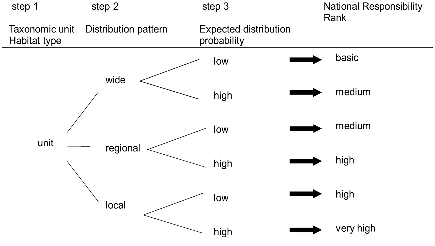
Decision tree for the determination of national responsibilities.
Habitats have both an inherent variability and variations in how they are interpreted from country to country, and sometimes between regions in the same country (
Definitions also differ between international organizations, such as FAO, CBD, and UNFCCC (
National habitat classifications are usually structured in a hierarchical order consisting of subclasses, which allows a detailed distinction of habitat types dependent on several variables. For example, the German classification, which was used to compile the Red List of German habitats (
International classifications, which are not restricted to specific habitat groups and covering a larger geographic range, have been published for Europe and the Palearctic. The CORINE (CORINE: Coordinated Information on the Environment;
The European Nature Information System (EUNIS; eunis.eea.europa.eu/) provides a database on habitats, species and protected areas which is built on a hierarchical habitat classification (
Annex I of the Habitats Directive lists habitats for which Sites of Community Interest (SCI) must designate sites as part of the NATURA 2000 network as SACs (
In the second step, the distribution pattern of the habitat unit is determined. Generally, the distribution pattern may serve as an approximation of the ability of a habitat to cope with threat factors, similar to a species’ distribution pattern in relation to environmental conditions (e.g.
For determining the distribution pattern, the choice of the biogeographical map needs to be considered. For the assessment of habitat distribution patterns across biogeographic regions, we have examined the following maps, (1) the Indicative European Map of Biogeographic Regions (hereafter IEMB;
The IEMB was produced to define the biogeographical regions mentioned in Art.1 c) (iii) of the Habitats Directive (Figure 2) and is the official geographical framework for which Sites of Community Interest are designated and for monitoring and reporting on habitat types (Article 17 reporting). The IEMB was formally adopted by the Habitats Committee, the body established to oversee the implementation of the Habitats Directive. It is based on interpretations of the “Map of Natural Vegetation of the Member Countries of the European Community and of the Council of Europe” and the “Map of the Natural Vegetation of Europe” (Noirfalse 1987, Bohn et al 2000,
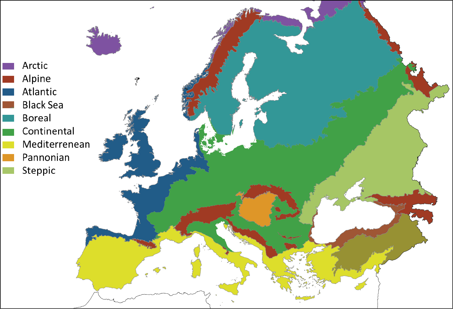
Indicative European Map of Biogeographic Regions (
In the 1960ies, the goal of establishing a worldwide network of natural reserves encompassing representative areas of the world’s ecosystems was widely supported (
Comparison of the four biogeographic maps.
| Udvardy’s system | Indicative European Map of Biogeographic Regions (IEMB) | Environmental Zones (ESE) | WWF Ecoregions | |
|---|---|---|---|---|
| Development | Developed for the IUCN between 1970-1975 by Dasman and Udvardy ( |
Scientific Working Group of the Habitats Directive, ( |
|
World Wildlife Fund for Nature, Olsen et al 2001a |
| Name of regions | Biogeographic provinces | Biogeographic regions | Environmental zones | Ecoregions |
| Basic principle | Combining ecoclimatic features and taxonomic differences, biogeographic provinces delineated by faunal regions and climax vegetation type | Based on “Map of Natural Vegetation” (Noirfalse 1987) & Map of Natural Vegetation of Europe. Vegetation units were allocated to biogeographical regions followed by generalization & simplication | Climatic stratification of the environment of Europe, based on statistical clustering of environmental variables | Delineations regarding species compositions, ecological dynamics, shared environmental conditions and, ecological interactions |
| Number of European regions | 14 | 8 | 13 | 44 |
| Number of (land) regions relevant for forest habitats | 13 | 7 regions for EU25, 9 for EU27, and 11 for Pan Europe. | 12 | 40 |
| Advantages | Consistent algorithms, not politically influenced | Widely accepted by policy makers | Scientific statistical approach not politically influenced, based directly on climatic variables, not vegetation | Not politically influenced |
| Weaknesses | Vegetation as determining factor | Border adjusted for administrative convenience vegetation as determining factor | Large number of regions, inconsistent delineation, based on vegetation |
A third map, the WWF ecoregions map (
The Environmental Stratification of Europe (hereafter called ESE;
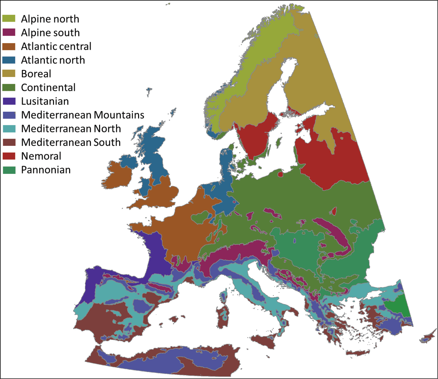
Environmental Zones of Europe (
Table 1 summarizes the characteristics, advantages, and disadvantages of the four maps. Vegetation is used as the main determining factor for delineating regions in all except the environmental stratification zones of
Comparison of the different biogeographic maps has shown differences between each of them, e.g. the number of biogeographic regions or environmental zones is not the same. Thus, habitats may occur in more zones when using fine-grained biographic zones than when using coarser grained maps. Moreover, as environments rarely have abrupt natural borders, any stratification will sometimes allocate similar environments on both sides of a border into different categories. This can result in habitats with small distributions occurring in 2 or more zones. For example, habitat 91R0, “Dinaric dolomite Scot’s pine forest (Genisto januenis-Pinetum)”, with a reported distribution area of 2885 km2 belongs to the 10 habitats with the smallest distribution ranges but is found in two zones of the IEMB map. The definition of classes of the distribution pattern used should reflect these aspects in such a way that the distribution of habitats across responsibility classes should not deviate too strongly from each other when different biogeographic concepts are used and should not allocate habitats with a small distribution area into a wide category. Here, we develop the categories for two maps, the ESE, as it has been widely accepted in habitat monitoring and is based on objective criteria for the delimitation of the different environmental zones, and the IEMB map, which has a legal status.
For the IEMB map, a local distribution pattern is attributed to habitats occurring in patches belonging to a single biogeographic region. Regional are habitats with a up to two-thirds of the distribution area in one biogeographic region. Wide refers to habitats with a distribution spanning two or more biogeographic regions.
For the ESE, a local distribution pattern is attributed to habitats occurring in only one environmental zone. Habitats have a regional distribution, if they are restricted to two neighboring environmental zones. All habitats with a distribution spanning three or more environmental zones were considered habitats with a wide distribution.
The third step of the proposed national responsibility method is to determine the expected value of occurrence (OVexp) in the focal area (e.g. a country). Following the suggestion of
The reference area should comprise the potential distribution area of a habitat in order to correctly determine whether the habitat distribution within a focal country plays a crucial role for the global persistence of a habitat or not. The main difficulty with this approach is data availability on habitat distribution and the different definitions, which exist world-wide. Also, different habitats will have different distributional limits so that whatever the reference area is some habitats will be included only incompletely or marginally. Several reference areas might be considered appropriate for European habitat types, 1) geographical Europe (Ural as eastern border; extent 10.936.779 km²), 2) the Western Palearctic (Europe, the Middle East, and North Africa, 33.225.342 km²), or 3) the Palearctic (including Europe, northern Africa, Russia, northern and central Asia, covering 54.244.453 km², see
Another important decision in this last step concerns the cut-off value. When can we consider an observed distribution probability as high or low? If the observed probability is twice as high as the expected value does this count as high? Given that the Agenda 2010 and the Aichi targets oblige European Member States to conserve a significant part of its biodiversity in each biogeographic region, this third and last step, as suggested here, should be conservative and accounts for the international importance of a habitat in a country and within a biogeographic region.
National responsibilities for EU forest habitats
As a test of the proposed methodology, we determined national responsibilities across geographical Europe, the Western Palearctic region, and the Palearctic region as reference areas and the ESE and IEMB maps for the 71 Annex I forest habitat types occurring in the EU25 (Table A4). We assessed national responsibilities using spatial datasets giving distribution of the habitats (
The highest number of forest habitat types was found in Italy (36 out of 71; 51%) followed by France (29, 41%), Spain (28, 39%) and Greece (27, 38%; Figure 4). The number of habitat types was positively correlated with the size of the country (R23 = 0.702; p < 0.001).
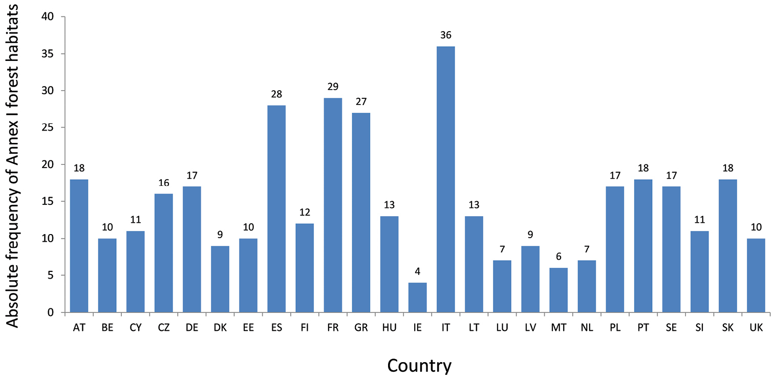
Number of forest habitat types as defined in the Annex I of the Habitats Directive by European country. The countries are abbreviated following the two-letter convention of the international community (ISO 3166-1 alpha-2 codes; AT = Austria, BE = Belgium, CY = Cyprus, CZ = Czech Republic, DE = Germany, DK = Denmark, EE = Estonia, ES = Spain, FI = Finland, FR = France, GR = Greece, HU = Hungary, IE = Ireland, IT = Italy, LT = Lithuania, LU = Luxembourg, LV = Latvia, MT = Malta, NL = Netherlands, PL = Poland, PT = Portugal, SE = Sweden, SI = Slovenia, SK = Slovakia, UK = Great Britain).
The distributions of natural responsibility (NR) classes largely resembled each other for the different combinations of reference area and biogeographic map. The most common rank in all cases was “medium”; the rank “very high” was the least common (Figure 5). We compared the number of NR-ranks of the six different combinations of reference area and biogeographic map using the combination Europe as reference area and the IEMB map as a baseline. The least affected rank in all the different assessments was the rank “very high”, which showed an N between 22 and 24. The largest differences were found for the “basic” rank. The number of this rank ranged between 59 and 134 (Figure 5). With increasing size of the reference area, a shift from allocations to a basic rank to allocations to a medium rank (from 1:4 to 1:1) was observed (Figure 6; Figure 7). The comparison of the allocation of habitats to responsibility classes between the two different biogeographic maps ESE and IEMB showed a shift from lower to higher ranks for all three reference areas, especially a shift from the ranks “medium” toward “high” (Figure 7), for the finer grained ESE map.
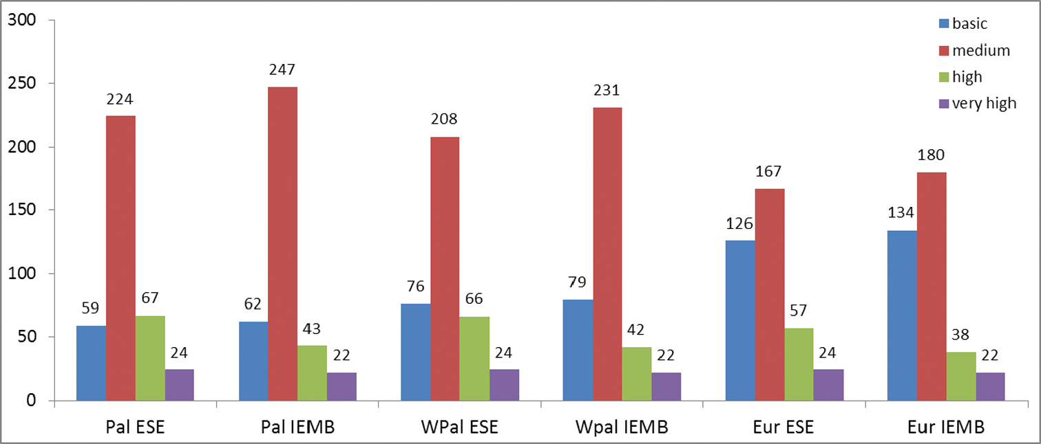
Distribution of National Responsibility ranks in the different combinations of reference area and biogeographic map. Reference area: Pal= Palearctis, WPal = Western Palearctis, Eur = geographic Europe; maps: ESE = Environmental zones, IEMB = IEMB biogeographic map.
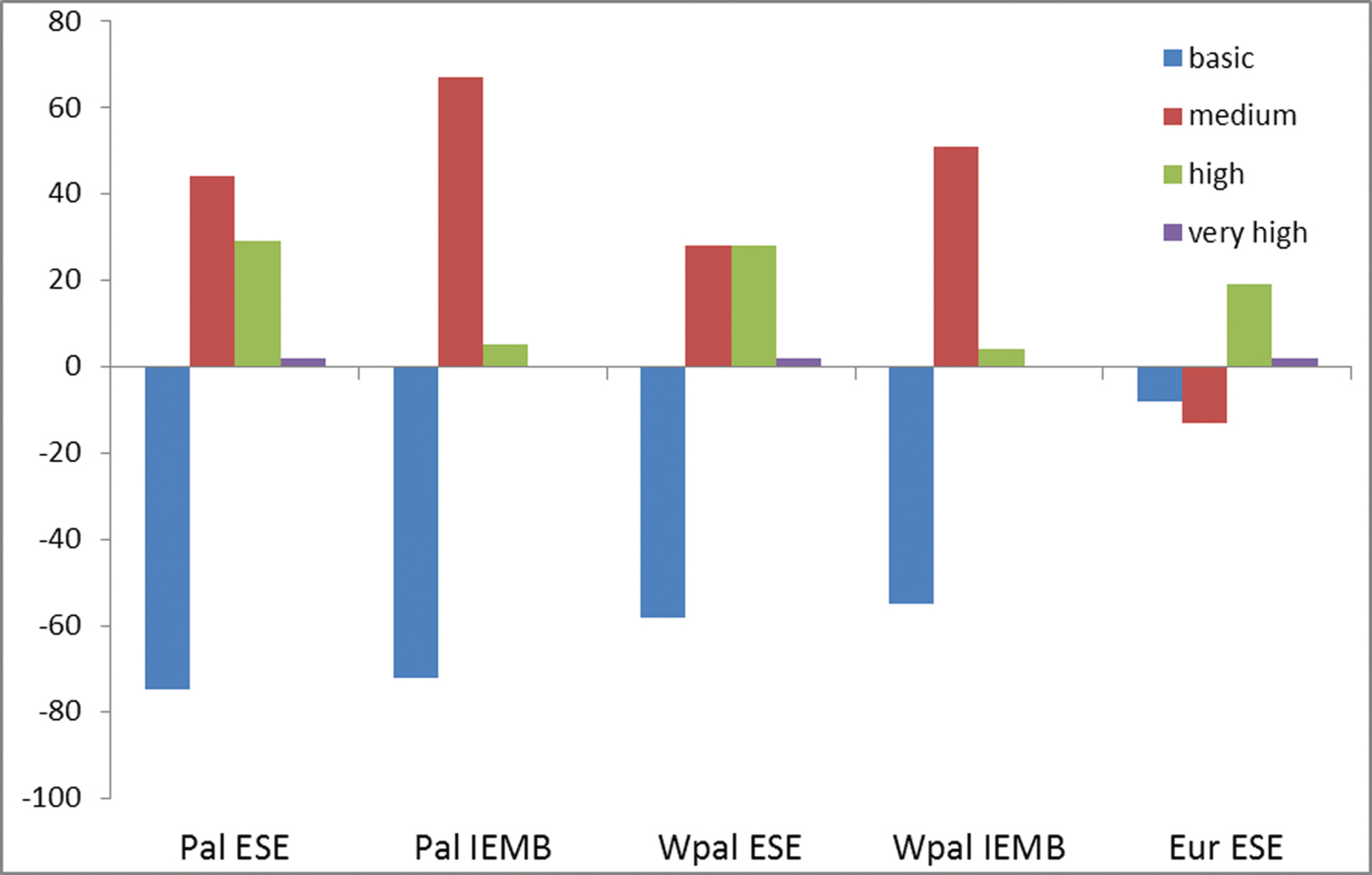
Differences in the National Responsibility-rank distribution between the assessments with Europe as reference area and the IEMB biogeographic map and the other 5 combinations (reference area: Pal= Palearctis, WPal = Western Palearctis, Eur = geographic Europe; maps: ESE = Environmental zones, IEMB = IEMB biogeographic map).
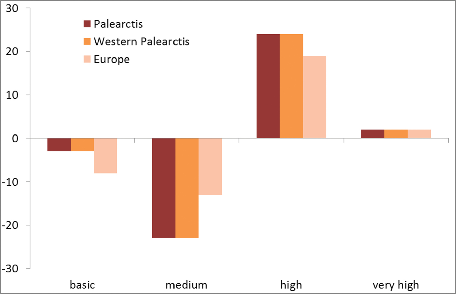
Shifts of the allocation of forest habitat types to responsibility classes when using the ESE versus the IEMB within each reference area.
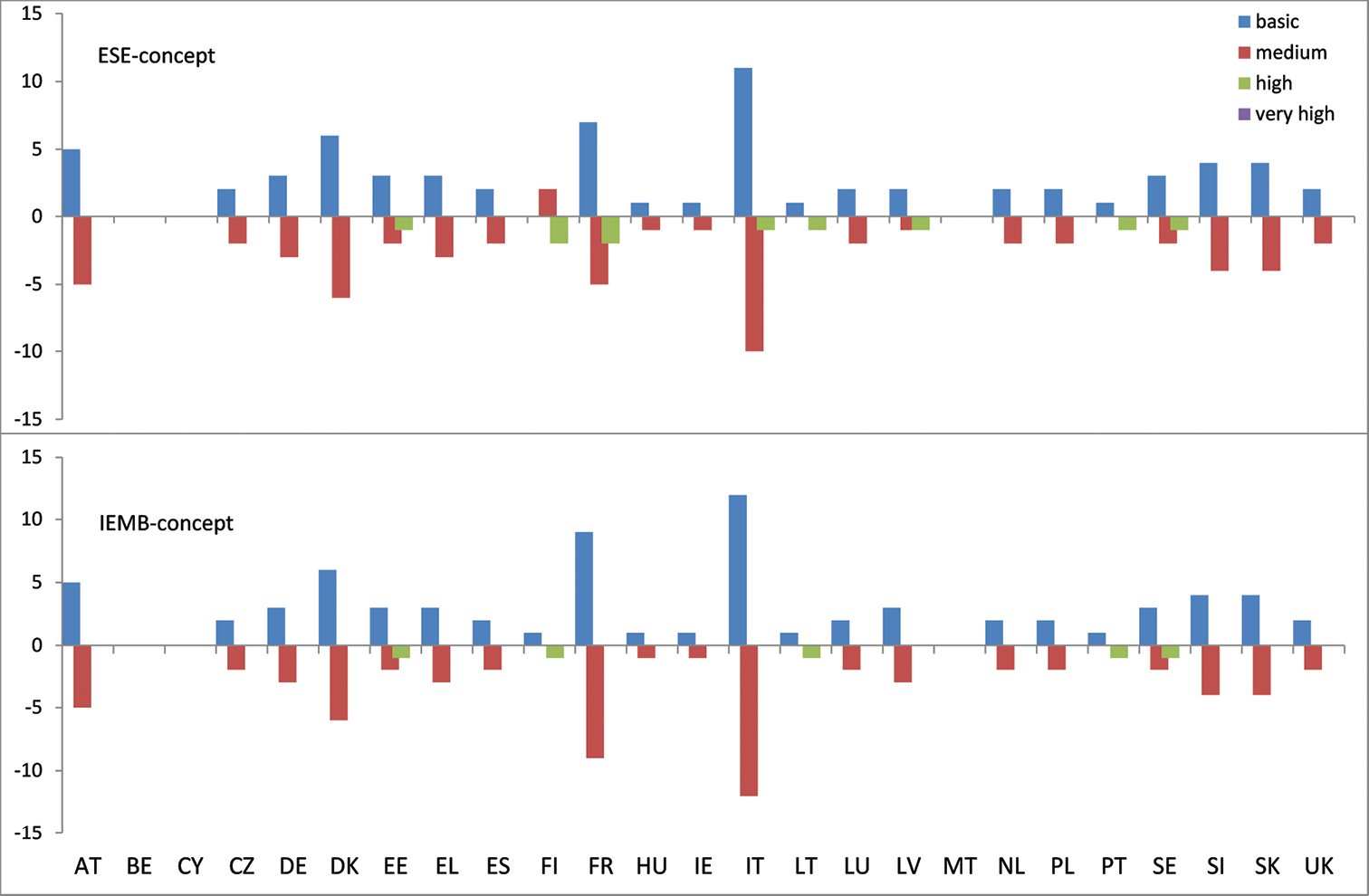
Comparing the two biogeographic maps by country reveals shifts mainly from medium to high ranks for northern countries (EE, LV, LT, FI, SE) and countries in the Mediterranean bioregion (ES, IT, FR, CY, PT). Changes were the least for countries in Central and Western Europe (BE, IE, LU, NL, PL, UK; Figure 8). We also found higher ranks with increasing size of the reference area (comparison of Palearctic Region to geographical Europe in Figure 9). The strongest shifts from basic to medium ranks were observed for AT, DK, FR, and IT.
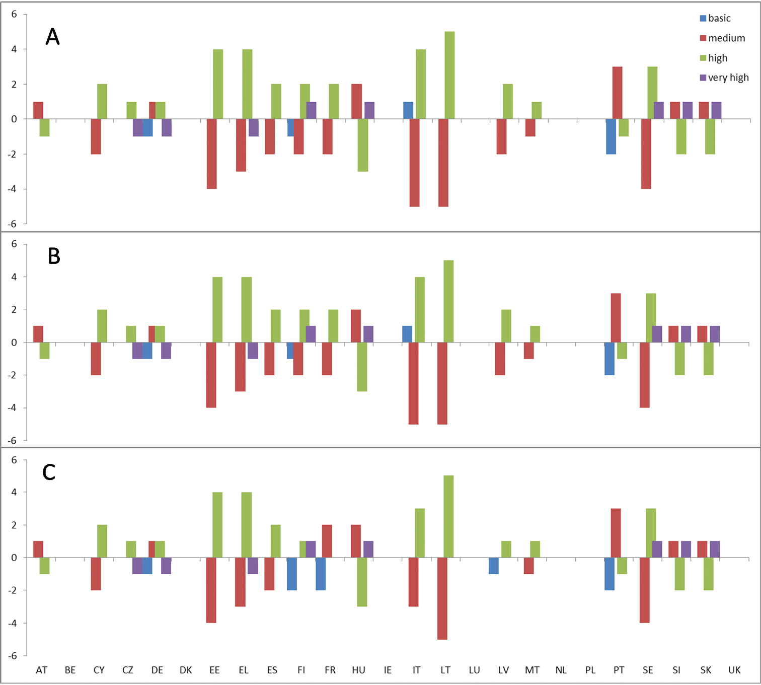
Shifts of the allocation of forest habitat types to responsibility classes per country when using the ESE versus the IEMB biogeographic map for the different reference areas: A=Palearctis; B = Western Palearctis; and C = Europe. The countries are abbreviated following the two-letter convention of the international community (ISO 3166-1 alpha-2 codes; AT = Austria, BE = Belgium, CY = Cyprus, CZ = Czech Republic, DE = Germany, DK = Denmark, EE = Estonia, ES = Spain, FI = Finland, FR = France, GR = Greece, HU = Hungary, IE = Ireland, IT = Italy, LT = Lithuania, LU = Luxembourg, LV = Latvia, MT = Malta, NL = Netherlands, PL = Poland, PT = Portugal, SE = Sweden, SI = Slovenia, SK = Slovakia, UK = Great Britain).
Shifts of allocations to ranks of national responsibility classes of countries when using the Palearctic versus Europe as reference area for the ESE and IEMB-maps. The countries are abbreviated following the two-letter convention of the international community (ISO 3166-1 alpha-2 codes; AT = Austria, BE = Belgium, CY = Cyprus, CZ = Czech Republic, DE = Germany, DK = Denmark, EE = Estonia, ES = Spain, FI = Finland, FR = France, GR = Greece, HU = Hungary, IE = Ireland, IT = Italy, LT = Lithuania, LU = Luxembourg, LV = Latvia, MT = Malta, NL = Netherlands, PL = Poland, PT = Portugal, SE = Sweden, SI = Slovenia, SK = Slovakia, UK = Great Britain).
A multiple regression of the differences in the rank “medium” between NR assessments based on the ESE map using as reference area the Palearctic region or geographical Europe (F2, 22 = 6.899; p = 0.005) showed a difference, but this difference was not explained by the size of a country (t22 = -1.304; p = 0.205). Differences were mainly driven by the number of habitats occurring within a country (t22 = 3.507; p = 0.002).
In the light of continuing decline of natural habitats (CBD 2010) and on-going biodiversity loss (
The method proposed here, while scientifically sound and relatively robust, suffers from two main issues related to the conservation of habitat types, 1) the lack of a globally and even regionally accepted habitat classification, and 2) the limited availability of distribution data across biomes, such as the Western Palearctic or the Palearctic in general. The first point impacts on the method in two ways, firstly, it restricts its usability to habitats with the same definition standard, and secondly comparability of national responsibilities of habitats with the same definition may not be totally correct, as important elements can differ in habitat types found e.g. in northern or central Europe due to environmental or ecological drift (e.g.
The aim of our method, however, is to create a globally applicable method to determine national responsibilities. Accepted habitat classifications and spatial information on their distribution are therefore urgently needed, as recommended in a recent article (
In conclusion, the methodology to determine national responsibilities presented here is readily applicable to determine conservation responsibilities for habitats of the EU25 countries. It should be based on the environmental stratification of Europe (ESE;
There are two more important problems, which need to be considered in the future, 1) the variability in the quality of a habitat and 2) the coherence of distribution data. The quality of a habitat type has not been homogeneously assessed across Europe, but may depend on management history, size, pollution and other factors. Our method can capture habitat quality by replacing the step on distribution pattern (as also suggested for the species method using abundance data) with a quality index. However, such data is not available widely and thus currently not applicable. Secondly, in the future, coherent distribution data, based on a consistent and complete habitat classification, should be gathered and made available across more countries than the EU25. Then, the methodology to determine national responsibilities has a unique potential to set, in combination with existing systems of threatenedness, such as Red Lists, conservation priorities (
This publication is a contribution from the project SCALES: Securing the Conservation of biodiversity across Administrative Levels and spatial, temporal, and Ecological Scales, funded under the European Union’s Framework Program 7 (grant 226852; www.scales-project.net;
Supplementary information to National responsibilities for conserving habitats - a freely scalable method. (doi: 10.3897/natureconservation.3.3710.app). File format: MS Word Document (docx).
Explanation note: The annex does provide a more detailed comparison of the different biogeographic maps. It further gives a list of all forest habitats given in the EU Habitats Direction.