


(C) 2013 Maj-Britt Pontoppidan. This is an open access article distributed under the terms of the Creative Commons Attribution License 3.0 (CC-BY), which permits unrestricted use, distribution, and reproduction in any medium, provided the original author and source are credited.
For reference, use of the paginated PDF or printed version of this article is recommended.
Citation: Pontoppidan M-B, Nachman G (2013) Spatial Amphibian Impact Assessment – a management tool for assessment of road effects on regional populations of Moor frogs (Rana arvalis). Nature Conservation 5: 29–52. doi: 10.3897/natureconservation.5.4612
An expanding network of roads and railways fragments natural habitat affecting the amount and quality of habitat and reducing connectivity between habitat patches with severe consequences for biodiversity and population persistence. To ensure an ecologically sustainable transportation system it is essential to find agreement between nature conservation and land use. However, sustainable road planning requires adequate tools for assessment, prevention and mitigation of the impacts of infrastructure. In this study, we present a spatially explicit model, SAIA (Spatial Amphibian Impact Assessment), to be used as a standardized and quantitative tool for assessing the impact of roads on pond-breeding amphibians. The model considers a landscape mosaic of breeding habitat, summer habitat and uninhabitable land. As input, we use a GIS-map of the landscape with information on land cover as well as data on observed frog populations in the survey area. The dispersal of juvenile frogs is simulated by means of individual-based modelling, while a population-based model is used for simulating population dynamics. In combination the two types of models generate output on landscape connectivity and population viability. Analyses of maps without the planned road constructions will constitute a “null-model” against which other scenarios can be compared, making it possible to assess the effect of road projects on landscape connectivity and population dynamics. Analyses and comparisons of several alternative road projects can identify the least harmful solution. The effect of mitigation measures, such as new breeding ponds and underpasses, can be evaluated by incorporating them in the maps, thereby enhancing the utility of the model as a management tool in Environmental Impact Assessments. We demonstrate how SAIA can be used to assess which management measures would be best to mitigate the effect of landscape fragmentation caused by road constructions by means of a case study dedicated to the Moor frog (Rana arvalis).
Rana arvalis, Individual-based modelling, Fragmentation, Connectivity, Pond-breeding amphibians, Landscape planning, mitigation, management tool, population persistence
Over the last decade a growing amount of literature has documented the severe impacts of transport infrastructure on biodiversity, population persistence and gene flow. An expanding network of roads and railways divides natural habitat into smaller and smaller fragments, affecting the amount and quality of habitat and reducing connectivity between habitat patches (
Movement is vital to the survival of animal populations. The persistence of a population depends on the amount and accessibility of its required resources and, within a metapopulation framework, also on sufficient dispersal between subpopulations (
We have developed a strategic management tool to be used in assessment and mitigation of road effects on a regional population of pond-breeding amphibians. The model, called SAIA (Spatial Amphibian Impact Assessment), combines the use of GIS land cover maps with IBM and provides information on connectivity as well as estimates of population persistence. SAIA is to be used by the Danish road authorities when assessing how new road constructions may affect Moor frogs (Rana arvalis). In this paper we demonstrate how SAIA can be used for assessing which management measures would be best to mitigate the effect of landscape fragmentation caused by the construction of a road ca 90 km west of Copenhagen, Denmark. To achieve this goal the following specific research questions were addressed:
- What is the structure of the regional habitat network before road construction?
- How is the habitat network affected by the new road?
- Which mitigation strategies are best suited to preserve the overall persistence of the regional population of Moor frogs?
SAIA combines an individual based model with a population based model. The individual based model provides estimates of landscape connectivity and immigration probabilities between all pair wise ponds. The population based model provides estimates of population size and persistence probability.
We use the terms dispersal and migration as defined by
Moor frogs spend most of their life in terrestrial habitat; aquatic habitat is only used during the breeding season in early spring (
Full model description following the protocol suggested by
List of variables characterizing the agents in SAIA.
| Variable | Notation | Value range | Agent type | Description |
|---|---|---|---|---|
| Area Value | W | 0.5; 1 | Cell | Effective area of the cell |
| Daily Survival | Ds | Cell | Daily survival probability | |
| Frog Density | D | Cell | Mean number of frogs in the cell | |
| Habitat Attraction | Ha | 1-5 | Cell | The cell’s relative attraction to frogs during movement |
| Habitat Code | Hc | Cell | The land cover category of the cell | |
| Habitat Survival | Hs | 1-5 | Cell | The cell’s relative survival index |
| Summer Quality | Hq | 1-5 | Cell | The cell’s relative suitability as summer habitat |
| Breeding Pond | Frog | Breeding pond of frog agents | ||
| Natal Pond | Frog | Natal pond of frog agents | ||
| Pond ID | Pond | ID number | ||
| Pond Perimeter | O | Pond | Perimeter of the pond | |
| Pond Quality | Q | 0.1-1 | Pond | Quality index of the pond |
| Population Size | N0 | Pond | Number of adult females (estimated as egg masses found in the pond during survey) | |
| Summer Habitat | A | Pond | Summer habitat cells associated with the pond | |
| Summer Habitat Area | A’ | Pond | Effective area of associated summer habitat |
To construct a model landscape in which our virtual frogs can move we use a GIS raster map of the study area with land cover data. Each raster cell contains information about the cell’s land cover or habitat type (Hc). Moreover, three variables are associated with each category of land cover/habitat (Table 2): Hq, the category’s relative suitability as summer habitat; Ha, the category’s relative attraction to frogs during movement and Hs, the category’s relative survival index. For each cell, the assigned survival index is converted into a daily survival probability (Ds). When concerning paved roads, the daily survival probabilities ranges between 0.1 and 0.8 depending on road category; all other land cover/habitat categories are assigned values between 0.9820 and 0.9995 (see Appendix in the supplementary material for details). Cells with structures or habitats which are assumed inaccessible to the frogs (e.g. buildings, fences or large water bodies) are given a habitat attraction of 1. This will prevent the frogs from entering the cell.
Land cover categories and the associated values of Habitat Survival, Habitat Attraction and Summer Quality.
| Habitat Code (Hc) | Description | Habitat Attraction (Ha) | Habitat Survival (Hs) | Summer Quality (Hq) |
|---|---|---|---|---|
| 2 | 4-lane motorway | 2 | N/A | 1 |
| 3 | 2-lane motorway | 2 | N/A | 1 |
| 4 | Road, width > 6m | 3 | N/A | 1 |
| 5 | Road, width 3-6 m | 3 | N/A | 1 |
| 6 | Other roads | 3 | 2 | 2 |
| 8 | Pathway | 4 | 4 | 3 |
| 10 | Multiple surface | 3 | 3 | 3 |
| 11 | Railway | 4 | 2 | 3 |
| 12 | Building | 1 | N/A | N/A |
| 15 | Other made surface | 2 | 3 | 2 |
| 18 | Wetlands | 5 | 5 | 5 |
| 20 | Running water | 4 | 4 | 3 |
| 22 | Meadows | 5 | 5 | 5 |
| 24 | Grassland | 4 | 4 | 4 |
| 25 | Lakes | 1 | N/A | N/A |
| 28 | Hedgerow | 4 | 4 | 4 |
| 29 | Heath land | 5 | 5 | 4 |
| 32 | Woodland | 4 | 4 | 4 |
| 34 | Stand of trees | 4 | 4 | 3 |
| 36 | Bare surface | 2 | 2 | 1 |
| 40 | Fallow land | 4 | 4 | 4 |
| 42 | Field crops | 2 | 2 | 2 |
| 50 | Drift fence | 1 | N/A | N/A |
| 60 | Underpass | 4 | 4 | 1 |
A point-data set containing information about potential breeding ponds found in the study area is used to create stationary pond agents. Each pond agent is characterized by an ID number, the perimeter of the pond (O), initial population size (adult females) (N0) and a quality index (Q) indicating the suitability of the pond and the immediate surroundings (20 m) in regard to egg and larval survival. In addition the pond variable A is updated with a list of summer habitat cells within migration distance. Summer habitat cells are identified as cells with SummerQuality (Hq) > 3. Summer habitat cells can be completely surrounded by other summer habitat cells (core cells) or have one or more neighbouring cells which are not summer habitat (edge cells). To account for edge effects, core cells are given an area value (W) of 1 while W is 0.5 for edge cells (
The IBM is largely identical to the model described in
At the start of a simulation, 250 frog agents are created at each pond. The frogs then disperse through the landscape in random directions from the ponds until they find suitable summer habitat; the movement of the frogs depends on the attractiveness of neighbouring cells and the cells’ suitabilities as summer habitat. Survival probabilities depend on the traversed habitat types. Unlike the former model, movement behaviour in SAIA also depends on weather conditions. A database containing data on daily precipitation (
After the individual based simulation, a population based model simulates the population dynamics in each pond through 40 iterations of a life cycle model. The elements of the life cycle model are 1) Reproduction, 2) Survival and 3) Immigration. For simplicity, we only model the female part of the population. We assume a sex ratio of 1:1 and that females always become mated once in a season. Pond populations are grouped by age from 0 through 6 years, and survival and reproductive rates are based on life-table data constructed by amphibian experts (
Life table for Rana arvalis constructed by amphibian experts.
| Stage/Age | Survival probability | Fecundity (eggs pr. female) |
|---|---|---|
| Egg/larvae | 0.005 | - |
| 0 | 0.55 | 0 |
| 1 | 0.55 | 70 |
| 2 | 0.55 | 945 |
| 3 | 0.55 | 1190 |
| 4 | 0.50 | 1250 |
| 5 | 0.40 | 1300 |
| 6 | 0.20 | 1300 |
Individuals can start reproducing in their third year. As in
At the end of the individual based simulation, the following output was recorded:
the number of surviving frogs, the natal and breeding ponds of all frogs, and the immigration probabilities (pij) between all pair-wise ponds. Landscape connectivity (S) is found as
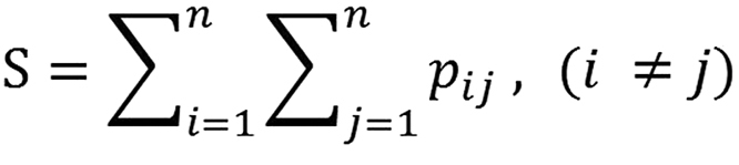 (eq. 1)
At the end of the population based simulation, the estimated population size of each pond is recorded as the resulting numbers of frogs of ages 2 through 6. The model was run 50 times and mean connectivity with 95% confidence intervals (CI) was computed. For each pond, we computed mean population size with 95% confidence intervals (CI). Pond persistence probability was computed as the proportion of replicates where the estimated population size was positive. The regional population size was computed as the sum of all ponds. Mean number of populated ponds with 95% CI was also calculated. SAIA’s connectivity measure is an index of the potential connectivity between all ponds, whether they are populated or not. The population based model links the potential connectivity with local population dynamics, and estimated abundances and persistence probabilities can be regarded as a result of the realised connectivity. The estimated landscape connectivity and population size are considered measures of the landscape's ecological performance in regard to the modelled species.
Cluster analysis was used to identify highly connected groups of ponds. Ponds were grouped into clusters depending on their mutual connectivity, using unweighted, arithmetic, average clustering as described by
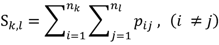 (eq. 2)
where nk and nl are the number of ponds in clusters k and l, respectively. Cluster abundance is computed as the sum of the member ponds’ estimated population size.
We have applied a bottom-up approach and used pattern oriented modelling (
We apply SAIA to a road project in Denmark and demonstrate the workflow of an impact assessment. The project concerns an area in the north-western part of Zealand, 10 km east of the city of Kalundborg (55°40.14'N, 11°17.85'E) (Figure 1) and includes a broadening of an existing 2-lane motorway into a 4-lane motorway as well as an extension of the motorway. The assessment procedure can be divided into three parts – Initial analyses, Mitigation planning and Mitigation analysis.
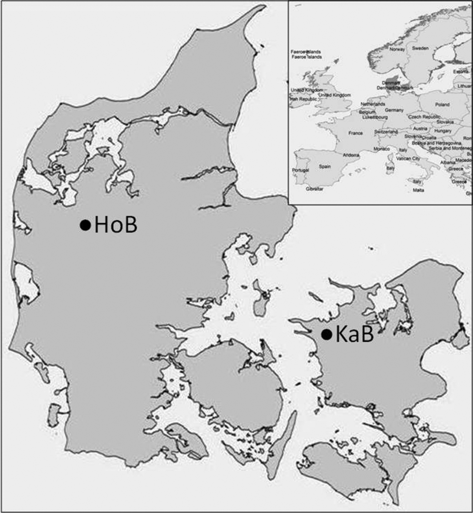
Location of two study areas in Denmark. KaB is an area near Kalundborg on Zealand and HoB is near Holstebro in Jutland. Only KaB is used in the present analysis, but both areas are used for the parameterisation of the model.
This part involves the construction and analysis of two maps. The first map, Scenario 0, is a map of the landscape as it looks before the planned road project. This map serves as Null Scenario and the results of the analysis are considered the state of the landscape we wish to maintain. The second map, Scenario 1, is of the landscape as expected after road construction. Analysis of this map gives indications of the effects the planned road construction can have on the ecological performance of the landscape.
Construction of the map is based on a GIS data set from the road project, supplied by the Danish Road Directorate and an environmental consultancy firm, Amphi Consult. The extent of the land cover map is 600 × 800 cells, and each cell is 10 × 10 m. All cells are assigned values of Ha, Hs and Hq depending on their land cover type, following a protocol designed by Amphi Consult (
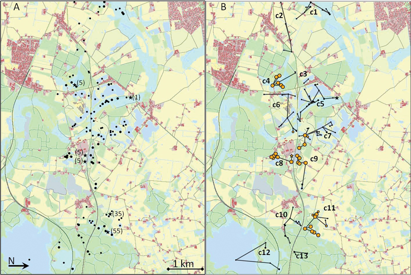
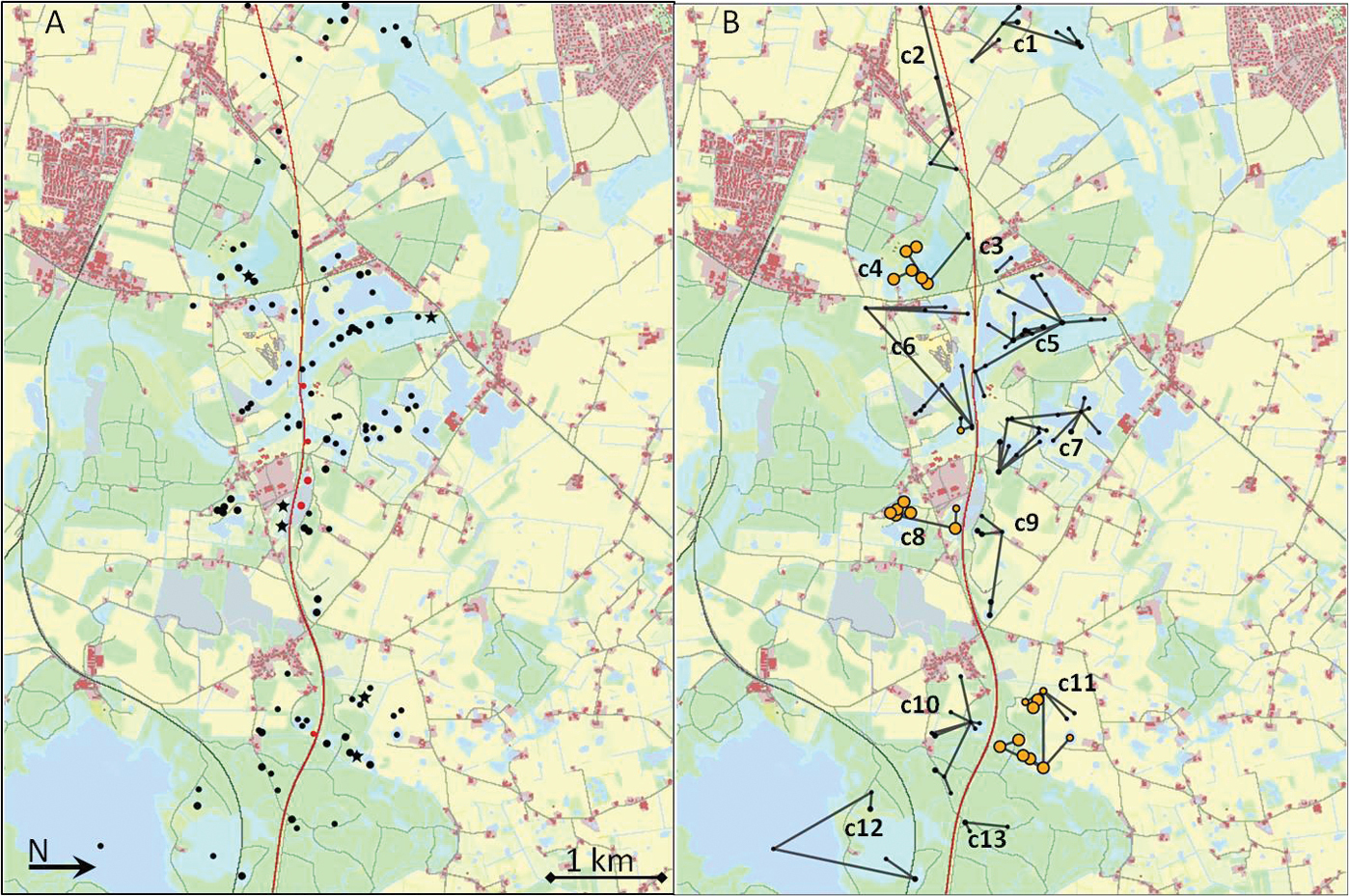
Scenario 0. A Map of the landscape before road constructions. Black dots represent potential breeding ponds. Small dots are ponds with pond quality (Q) ≤ 6; large dots are ponds with Q ≥ 7. Populated ponds are indicated with a star shape. The number of egg masses found in the pond is shown in parenthesis B Result of cluster analysis showing clusters c1–c13. Ponds linked with black lines belong to the same cluster. Pond size and colour indicate the result of the population based model. Yellow circles represent ponds with an estimated population size ≥ 1. Ponds with larger yellow circles have a persistence probability > 0.75.
The map used in Scenario 0 is modified by changing the land cover category of the existing road section from a 2-lane motorway to a 4-lane motorway. The new section of the road is added as well and categorised as a 4-lane motorway (Figure 3A). As a consequence of the change in land cover category the daily survival probability (Ds) of the road cells decreases from 0.20 to 0.10 (Table A5 in the Appendix). The road construction also involves removal of five unpopulated ponds along the road (Figure 3A).
Scenario 1. A Map of the landscape after road constructions (red road). Black dots represent potential breeding ponds. Small dots are ponds with pond quality (Q) ≤ 6; large dots are ponds with Q ≥ 7. Populated ponds are indicated with a star shape. Pink ponds are ponds removed in connection with the constructions B Result of cluster analysis showing clusters c1–c13. Ponds linked with black lines belong to the same cluster. Pond size and colour indicate the result of the population based model. Yellow circles represent ponds with an estimated population size ≥ 1. Ponds with larger yellow circles have a persistence probability > 0.75.
Once the analyses of Scenario 0 and Scenario 1 are done, planning of possible mitigation measures can start. The results from the initial analyses can give insights in the structure of the pond network and can locate areas or subpopulation where the road construction will have the strongest impact. Likely source populations and their colonisation potential may be identified and possible sink population may be recognised. Interpretation of the results provides a basis for considerations about which mitigation measures are needed and where to place them. A series of scenarios with different suggestions for mitigation measures can then be constructed and analysed.
In this case study we construct and analyse three alternative mitigation scenarios - Scenario 2, Scenario 3a and Scenario 3b. The choices of mitigation measures depend as just mentioned on the results of the initial analysis. Thus, the reasoning behind the different mitigation scenarios will be explained in the result section. However, the map construction of the three scenarios is briefly described below.
In this scenario we add three underpasses to the map used in Scenario 1. Drift fences are established along the road for 100 m on each side of the underpass, except for underpass 2 which has a 300 m drift fence to the east. The location of the underpasses is shown in Figure 4A. Underpasses are constructed by changing the habitat code and the associated values of habitat attraction (Ha) and daily survival probability (Ds) of the affected road cells. Drift fences are created by changing the habitat attraction of the affected road section to 1, thus preventing access to the cells.
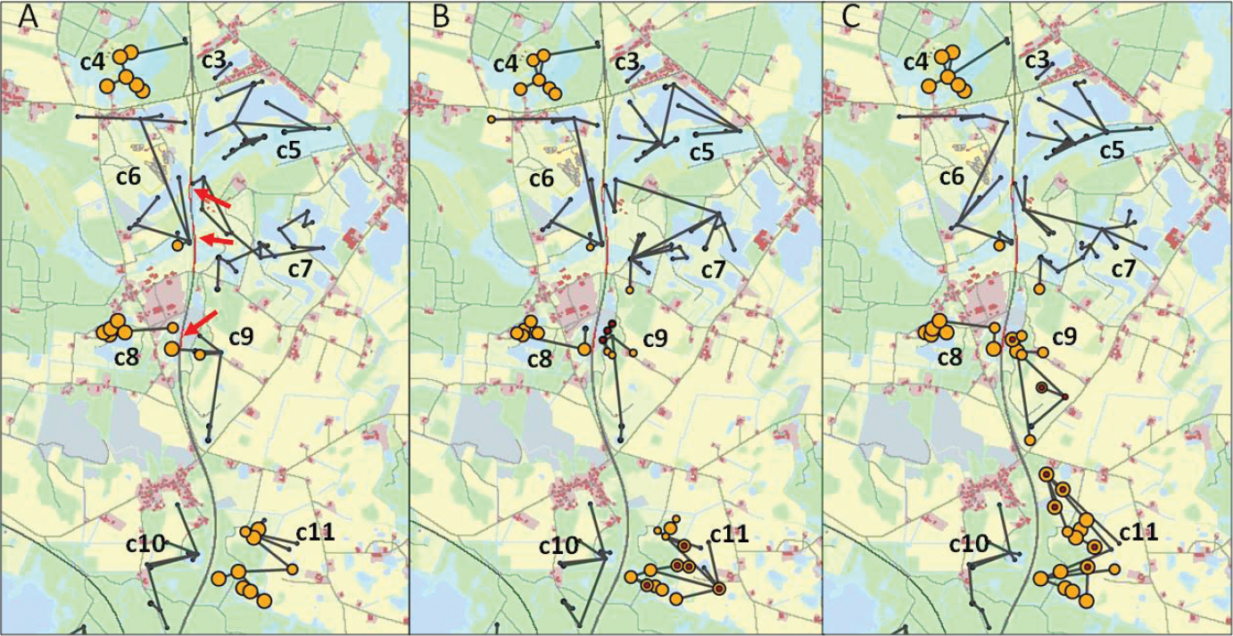
Analyses of mitigation measures. Result of cluster analyses showing clusters c3–c11. Ponds linked with black lines belong to the same cluster. Pond size and colour indicate the result of the population based model. Yellow circles represent populated ponds. Ponds with larger yellow circles have a persistence probability > 0.75. A Scenario 2 - Location of underpasses is shown with red arrows B Scenario 3a – Three new ponds in cluster c9 and five new ponds in c11 are shown with red dots C Scenario 3b – Eight new ponds connecting c9 and c11 are shown with red dots.
In these two scenarios eight artificial, high quality breeding ponds are added to the map used in Scenario 1. Scenario 3a and 3b represent two alternative locations of the eight ponds (Figure 4B and C). Each breeding pond is created as a pond agent and assigned a pond quality (Q) of 0.7. The initial population size (N0) is set to 0. The pond perimeter (O) is set to 79 m, corresponding to the average size of a standard artificial breeding pond.
The average percentage of ponds populated during a simulation is 32%, although only 22% of the ponds have a more permanent status (pond persistence probability > 0.75). The regional abundance of adult female frogs is estimated to be 157; the percentage of frogs surviving during dispersal is 57 %, and landscape connectivity is 55 (Figure 5). The cluster analysis groups the 121 ponds into 13 clusters, cluster sizes ranging from 2-20 ponds (Figure 2B, Table 4). The six populated ponds found during field surveys are distributed on four different clusters. One pond with only one adult female is found in cluster c5. Another pond, with an initial population of five, belongs to cluster c4 and two other ponds, also with a N0 of five, are found in cluster c8. Cluster c11 contains the remaining two populated ponds with an initial total population of 90 adult females. Apart from cluster c5, all of these initially populated clusters exhibit high viability. Clusters c4, c8 and c11 have mean pond persistence probabilities between 77% - 93% and estimated cluster abundances from 23–51 adult females. Cluster c9 also shows high values of abundance and persistence. Although initially unpopulated, c9 contains several high quality ponds and is connected with c8 and c11 which may promote colonisation and establishment. In cluster c6 and c7, the mean pond persistence probability is considerably lower (29–35%) as is the estimated cluster abundance. While the two clusters, especially c6, are connected with other populated clusters, they lack high-quality ponds and the clusters may function as sinks. In the remaining clusters the estimated abundance is less than one individual.
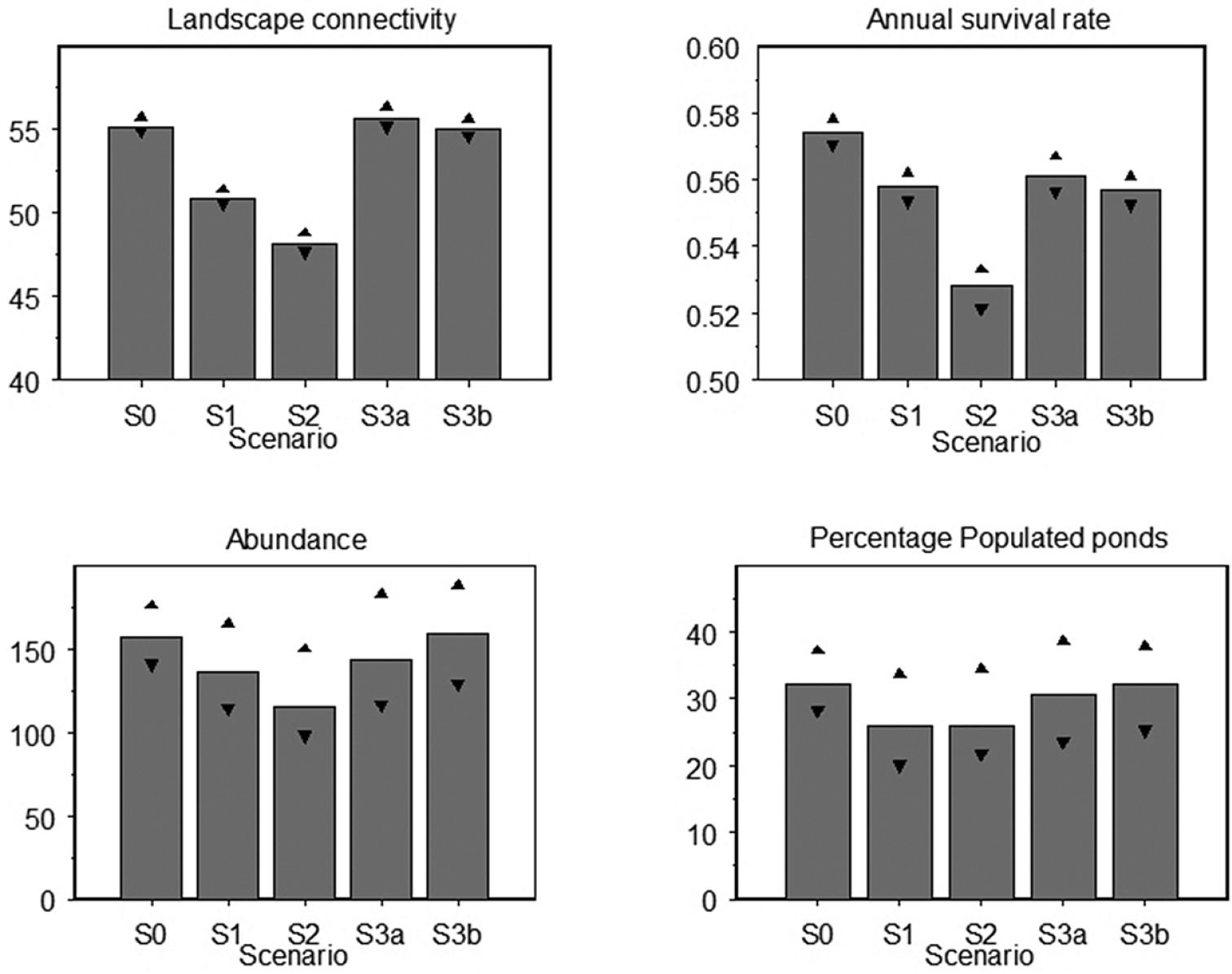
Key results from analysis of the five scenarios. Upper and lower 95% confidence limits are indicated with black triangles.
Results from analysis of Scenario 0 (before road construction).
| Cluster ID | c1 | c2 | c3 | c4 | c5 | c6 | c7 | c8 | c9 | c10 | c11 | c12 | c13 |
|---|---|---|---|---|---|---|---|---|---|---|---|---|---|
| Number of ponds in cluster | 9 | 5 | 2 | 8 | 20 | 13 | 19 | 7 | 7 | 11 | 12 | 5 | 3 |
| Number of high quality ponds (Q > 0.6) | 2 | 0 | 0 | 4 | 2 | 0 | 1 | 7 | 3 | 0 | 3 | 1 | 0 |
| Connectivity to other clusters | 0.45 | 0.54 | 0.30 | 0.57 | 2.19 | 1.13 | 2.94 | 0.36 | 1.20 | 0.07 | 0.10 | 0.05 | 0.06 |
| Estimated cluster abundance | 0 | 0 | 0 | 49 | 0 | 3 | 11 | 23 | 14 | 0 | 51 | 0 | 0 |
| Mean pond persistence probability | 0 | 0 | 0 | 0.82 | 0.03 | 0.29 | 0.35 | 0.93 | 0.73 | 0.01 | 0.77 | 0 | 0.13 |
| Connectivity to c4 | 0 | 0.09 | 0.04 | - | 0.01 | 0.44 | 0 | 0 | 0 | 0 | 0 | 0 | 0 |
| Connectivity to c8 | 0 | 0 | 0 | 0 | 0 | 0.23 | 0.04 | - | 0.10 | 0 | 0 | 0 | 0 |
| Connectivity to c11 | 0 | 0 | 0 | 0 | 0 | 0.00 | 0 | 0 | 0.02 | 0.02 | - | 0 | 0.06 |
After construction of the road, the percentage of populated ponds is reduced to 26% and the number of ponds with a persistence probability > 0.75 is now down to 16%. Survival rate of dispersing frogs is 56% and estimated regional abundance is 136 adult females. Landscape connectivity decreases to 51 (Figure 5). The number of clusters is unchanged but connectivity between clusters is reduced (Table 5). Connectivity from c7 and c9 to their primary source (c8) decreases more than 80%. Moreover, three ponds are lost in c7 and c9 due to the road construction. Estimated abundance and mean pond persistence probability decreases in c7 and c9 and these clusters are no longer able to uphold viable populations (Figure 3B). However, the initially populated clusters c4, c8 and c11 are not affected by the road construction.
Results from analysis of Scenario 1 (after road construction).
| Cluster ID | c1 | c2 | c3 | c4 | c5 | c6 | c7 | c8 | c9 | c10 | c11 | c12 | c13 |
|---|---|---|---|---|---|---|---|---|---|---|---|---|---|
| Number of ponds in cluster | 9 | 5 | 2 | 8 | 19 | 13 | 17 | 7 | 6 | 9 | 12 | 5 | 3 |
| Number of high quality ponds (Q > 0.6) | 2 | 0 | 0 | 4 | 2 | 0 | 1 | 7 | 2 | 0 | 3 | 1 | 0 |
| Connectivity to other clusters | 0.02 | 0.10 | 0.27 | 0.52 | 1.69 | 0.67 | 1.92 | 0.23 | 0.55 | 0.06 | 0.09 | 0.05 | 0.06 |
| Estimated cluster abundance | 0 | 0 | 0 | 50 | 2 | 2 | 1 | 24 | 5 | 0 | 49 | 0 | 0 |
| Mean pond persistence probability | 0 | 0 | 0.03 | 0.84 | 0.05 | 0.24 | 0.08 | 0.93 | 0.26 | 0 | 0.78 | 0 | 0.15 |
| Connectivity to c4 | 0 | 0.08 | 0 | - | 0 | 0.44 | 0 | 0 | 0 | 0 | 0 | 0 | 0 |
| Connectivity to c8 | 0 | 0 | 0 | 0 | 0 | 0.20 | 0.01 | - | 0.02 | 0 | 0 | 0 | 0 |
| Connectivity to c11 | 0 | 0 | 0 | 0 | 0 | 0 | 0 | 0 | 0.03 | 0 | - | 0 | 0.06 |
The initial analyses reveal that the landscape contains three viable populations (c4, c8 & c11) centred on the initially populated ponds. These populations appear not to be affected by the road construction and in the simulations the clusters seem to function as sources enabling colonisation and establishment of populations in c9 and c7. Cluster c4 has a large and viable population, but even though it is well connected with the neighbouring clusters their qualities are not high enough to enable establishment of new populations. Since c4 is not connected with c7 and c9, its potential as source cluster is low. Cluster c8 seems to be the primary source cluster to c9 and c7; however, expansion of the road heavily reduces its value as a source. Furthermore, the removal of three ponds between c9 and c7 may diminish the connectivity between these clusters. Cluster c11 has a viable population and although situated somewhat remotely there is still some connectivity to c7 and c9.
The results indicate that, in order to compensate or mitigate the effect of the road project, the best strategies will be either to re-establish connectivity across the road between cluster c8 and clusters c7/c9 and between cluster c7 and c9 or to take advantage of the viability of cluster c11 and its source potential. Based on this, we create and analyse the following scenarios:
Scenario 2: Connectivity across the road is re-established by constructing three underpasses and drift fences along the middle section of the motorway (Figure 4A). Two of the underpasses (including drift fences) were placed between cluster c6 and c7; the third between cluster c8 and c9. The expectation is that connectivity between cluster c8 and c9/c7 will improve and enable establishment of populations in cluster c9.
Scenario 3a: The quality of cluster c9 and c11 is improved by establishing three, and then five, new high quality ponds within the range of the clusters (Figure 4B). The three new ponds in cluster c9 are expected to improve the probability of successful establishment of immigrants as well as reconnect c9 with c7.We expect an increase in abundance in cluster c11, and hence increased immigration to and colonisation of cluster c9.
Scenario 3b: In this modification of Scenario 3a the quality of cluster c9 and c11 is still improved but with only one and two ponds, respectively. The remaining five ponds are used to create a dispersal corridor between cluster c11 and c9 (Figure 4C). This strategy is expected to enhance the abundance in cluster c11 and to improve connectivity to c9, thereby increasing the probability of colonisation.
Quite unexpectedly, the creation of drift fences and underpasses do not improve the condition of the landscape. The mean percentage of populated ponds is 26% and the percentage of ponds with persistence probability > 0.75 is 16% as in Scenario 1. However, the estimated regional abundance of female adults decreases to 115, landscape connectivity is 48 and dispersal survival rate 53% (Figure 5). As expected, connectivity between c8 and c9 is greatly improved. Cluster c9 now spans the road and has annexed one of the ponds in the periphery of c8 (Figure 4A). Abundance and mean pond persistence probability of cluster c9 increase; this, however, is due to the inclusion of a pond from cluster c8. Persistence and abundance do not improve on the original configuration of cluster c9 (Table 6). Apart from cluster c9, connectivity between initially populated clusters and other clusters does not improve. Connectivity to cluster c4 and c11 is unchanged, while connectivity to cluster c8 actually decreases. Finally, the abundance of frogs in cluster c4 and c11 decreases to 20% even though connectivity both within the cluster and to other clusters is unchanged.
Results from analysis of mitigation measures. Scenario 2: Drift fences and underpasses; Scenario 3a: Implementing new ponds in clusters c9 and c11; Scenario 3b: Implementing new ponds as corridor between c9 and c11.
| Cluster ID | Estimated cluster abundance | Mean pond persistence probability | Connectivity to c8 | Connectivity to c11 | ||||||||
|---|---|---|---|---|---|---|---|---|---|---|---|---|
| S2 |
S3a | S3b | S2 |
S3a | S3b | S2 |
S3a | S3b | S2 | S3a | S3b | |
| c4 | 40 | 48 | 49 | 0.82 | 0.82 | 0.82 | 0 | 0 | 0 | 0 | 0 | 0 |
| c7 | 1 | 3 | 4 | 0.08 | 0.11 | 0.11 | 0.002 (0.004) | 0 | 0 | 0 | 0 | 0 |
| c8 | 17 (21) | 23 | 23 | 0.90 (0.95) | 0.90 | 0.92 | - | - | - | 0 | 0 | 0 |
| c9 | 6 (2) | 11 | 10 | 0.38 (0.27) | 0.44 | 0.58 | 0.19 (0.29) | 0.02 | 0.02 | 0.025 | 0.03 | 0.22 |
| c11 | 40 | 50 | 61 | 0.74 | 0.80 | 0.85 | 0 | 0 | 0 | - | - | - |
* In Scenario 2 one pond originally belonging to c8 is annexed by c9. Entries in parentheses are values based on the original cluster configurations.
Establishment of eight new ponds has a positive effect on landscape condition. The estimated number of adult females in the region increases to 143, percentage of populated ponds is 31% and 19% of the ponds are permanently populated. Landscape connectivity is 56 and dispersal survival rate 56% (Figure 5). The five new ponds in cluster c11 perform well and contain permanent populations. However, the performance of the cluster does not improve, apart from a slightly higher persistence probability (Table 6). Cluster c9 seems to benefit from the additional ponds, although none of the new ponds contain permanent populations. Cluster abundance and connectivity are nearly restored to their original conditions although mean pond persistence probability is still below 50%. Connectivity from cluster c7 to other ponds improves somewhat, but not enough to restore the cluster to its former performance (Figure 4B).
With this strategy we succeed in restoring the landscape to its original ecological performance. The number of adult female frogs in the region is 159. Mean percentage of populated ponds is 32% and 22% are populated permanently. Dispersal survival rate is 56% and landscape connectivity is 55 (Figure 5). Three of the new ponds are now part of cluster c9 while the remaining five new ponds belong to cluster c11. Connectivity between cluster c9 and c11 is strong and six of the new ponds contain permanent populations (Figure 4C). The abundance and mean persistence probability of cluster c11 increase and are now better than before the road construction. Conditions in cluster c9 also improve, compared to Scenario 1, but its original performance is not quite restored. The performance of cluster c7 does not change and is still at the same level as found in Scenario 1 (Table 6).
This study demonstrates how initial analyses of the landscape before and after the planned road constructions can help to identify which areas will be most affected by the construction. The analyses enable the user to recognise the colonisation potential of the clusters and to identify source or sink clusters and to use this knowledge for planning mitigation measures. In the present case study, the simulations indicated that the six populations recorded during the field survey will be largely unaffected by the road construction. Nevertheless, the road construction will severely impair the colonisation potential of cluster c8, thereby reducing the ecological performance of the landscape. Of the three mitigation strategies tested, the analysis showed that Scenario 3b is the best solution. This strategy of connecting clusters c9 and c11 restores the landscape to its former ecological performance. Even though not all individual ponds or clusters will be in the same condition as before, the strategy promotes viable populations on both sides of the road. The strategy is not strictly aimed at mitigating the impaired connectivity across the road, but rather tries to compensate for the effects of road construction by improving other areas. Still, the populations on either side of the road are not totally isolated from each other; some dispersal does take place making genetic exchange possible.
Comparing the results from the analyses of Scenarios 3a and 3b suggests that the location of compensating new ponds is not trivial. In both scenarios cluster c11 gets five new ponds, all of high quality. Nevertheless, the results differ quite a lot. Scenario 3a places the new ponds within the cluster sharing the summer habitat of other ponds. Even though the new ponds are colonized and support viable populations, the abundance of frogs within the cluster does not improve. In Scenario 3b, where the abundance of frogs within cluster c11 increases, the new ponds were placed between c9 and c11 and only partly share summer habitat with other ponds. This result emphasizes that for the Moor frog the carrying capacity of an area is not improved by adding new ponds, only new or better summer habitat can achieve this. Hence, we may improve cluster performance by creating new ponds in unutilized summer habitat within dispersal distance.
In Scenarios 3a and 3b, cluster c9 is also enlarged with three new ponds. In these cases there was no difference in frog abundance in the cluster whether the new ponds were placed in unused summer habitat or not. In both scenarios, though, mean pond persistence probability greatly improved compared to Scenario 1. So, while adding ponds to a cluster did not improve carrying capacity, it ensured a more viable cluster population.
The analysis of Scenario 2 showed that drift fences and underpasses have negative effects on the ecological performance of this landscape. This result is highly surprising as well as controversial since fences and underpasses are standard mitigation measures used in many road projects (
Very little is known about the effects of mitigation measures on connectivity and local and regional population persistence. Once mitigation measures are implemented, efforts are seldom put into discovering how well they work. Recordings of animals using wild life passages reveal nothing about effects on local and regional persistence (
When planning road constructions, it is important to integrate mitigation measures right from the start. Often there are economic constraints on which measures are possible, certain structures as viaducts or bridges may already be in place or land available for compensation measures is restricted. SAIA offers a tool to evaluate different scenarios to find the best combination of mitigation measures for a given set of conditions. The model is meant to be used by non-specialists – all that is needed are GIS maps of the different scenarios. We attempted to find a balance between detailed and yet intuitive and easy interpretable output. Even though SAIA was developed for the Danish Road Directorate, its use is not restricted to road constructions but can be applied to other structures affecting the landscape and their potential impacts on wildlife.
The work was funded by the Danish Road Directorate. We thank Amphi Consult for providing us with amphibian expertise and field data. We are grateful for continuous and enthusiastic feed-back from M. Ujvári, M. Hesselsøe, A. Jørgensen and M. Schneekloth during model development. Special thanks are due to Uta Berger for encouraging and inspiring discussions. We thank Michal J. Reed for linguistic assistance. We also wish to thank two anonymous reviewers for insightful comments.
Full model description following the protocol suggested by