The fisheries examined in this study are located in the Sistan and Baluchestan Province (SBP) situated at the northern end of Mokran Sea (Gulf of Oman) in Iran (Pakzad et al. 2014). There are ten ports along a 270 km (167.77 miles) stretch of coastline from Govater Bay in the East to Kereti Bay in the West, spanning a longitude 59°13'E to 61°13'E (Figure 1).

Figure 1. 

Study area and the locations of fishing landing ports related to small scale fishing vessels.

Based on the local reportage of PFDSB and IFO, the fishery is an important source of income, cultural heritage and recreation in the area. In addition, it forms the largest employment with over 24,500 locals involved in fishing industries permanently or seasonally. The fishing system of SBP consists of inshore fleets, with 60% (1430) of vessels registered as weighing at least three gross tonnes, as most of which are primarily made of fibreglass. The fishing activities are mainly seasonal and fishermen change their fishing gear (gill nets, hand-lines/hook-and-lines and traps) and strategies based on water levels, habitats, migration patterns and species targeted. However, the majority of vessels that fish annually use gill nets. The total catches of the fourteen species examined in this study from 21 March 2015 to 18 March 2016 were 35,937 metric tonnes. This catch comprises 49% of the demersal fish catch; 31% of all fish species caught and 187 million US$ of economic value which represents an important resource for the fishery.

Nine years (21 March 2006 to 18 March 2015) of fisheries-dependent commercial landings and effort data for the fourteen demersal fish species listed earlier were acquired from Iran’s National Fishery Data Collection and Reporting System Unit and also reports from the Provincial Fisheries Department. In addition, the used time series of catch and standardised CPUE values as relative abundance indices are considerable as the supplementary data. The nominal CPUE indices that derived from commercial fisheries’ logbooks are affected by some variables such as spatiotemporal and environmental factors. The considered standardised CPUE indices are reliable abundance indices which allow the implementation of the conservation and management measures and have been obtained by the most common and competent statistical approach in the domain of fisheries’ researches, such as generalised additive models (GAMs), that are used for standardising catch and effort data.

Biomass dynamic models are popularly used for stock assessment when only catch and effort time series data are accessible (Hilborn and Walters 1992; Kinas 1996; Laloë 1995; Mäntyniemi et al. 2015; Quinn and Deriso 1999). These models equate current biomass as previous biomass plus surplus production (growth, recruitment and natural mortality) minus harvest removals (Hilborn and Walters 1992; McAllister and Kirkwood 1998; Schaefer 1957).

The biomass dynamics model of the equation discrete time form is as follows (Hilborn and Walters 1992):

B_t = B_t–1+ h (B_t–1) – C_t–1 (1)

In Equation 1, B_t–1, C_t– and h (B_t–1) denote biomass and catch for year t–1 and the surplus production function, respectively.

Bayesian state-space models consist of three levels (Berliner 1996; De Valpine and Hastings 2002; Haddon 2010; Parent and Rivot 2012) as follows:

(I) a process equation which depicts the time dynamics of a stochastic process as a function of time-invariant hyper-parameters. (II) an observation equation based on population-specific inspection data that are a function of the unobserved state process (Buckland et al. 2004). (III) the prior distributions level that comprises an explanation of the prior probability distribution of the parameters and condition at the first time moment (Rankin and Lemos 2015). These three levels are specified in the following section in the background of a surplus production model.

With regards to the Equation 1, the process equation describes the surplus production function in a generalised surplus production model (GSPM) (Fletcher 1978; Pella and Tomlinson 1969) as follows:

h (B_t–1) = r B_t–1(1 – (B_t–1 / K)^z), r > 0, K > 0, z > 0 (2)

where r is the intrinsic population growth rate; K is the carrying capacity of the population and z is the shape parameter of the production model that determines at which B/K ratio maximum surplus production was attained and commonly noted as equivalent biomass and at which the maximum sustainable yield (MSY) was attained (B_MSY). If the shape parameter was less than unity (0 < z < 1), then surplus production would increase (to the peak point) when the biomass was below K/2 (a left-skewed production curve). If the shape parameter was greater than unity (z > 1), then biomass production would increase (to the peak point) when the biomass was more than K/2 (a right-skewed production curve). If the shape parameter was identical to unity (z = 1), the production model would reduce to the Schafer form, attaining MSY when biomass was equal to K/2. If z approached zero (z → 0), the production model would reduce to the Fox model that results into maximum surplus production at ~0.37K.

Replacing Equation 2 in Equation 1 and multiplying the right hand side of the resultant equation with u_t yields the stochastic form of the biomass dynamic model with generalised surplus production (GSP) (Parent and Rivot 2012):

B_t = (B_t–1 + r_tB_t–1(1 – (B_t–1 / K)^z) – C_t–1)u_t (3)

Where u_t is process noise – supposed to be independent and log-normally distributed; specifically u_t = e^εt where ε_t ~ N[0, σ²], i.e. ε_t is i.i.d. normal with mean zero and variance σ².

Equation 3 was re-parameterised using relative biomass (P = B_t / K) to diminish parameter confounding such as that between biomass and K that could result in related priors (Meyer and Millar 1999) as follows. Thus, the final stochastic form of the process equation is given by Equation 4:

P_t = (P_t–1 + r_tP_t–1(1 – (P_t–1)^z) – C_t–1 / K)u_t (4)

According to regular assumptions, CPUE values are relative abundance indices proportional to the biomass. The observation equation relates the unobserved states B_t to the relative abundance indices I_t (Harley et al. 2001; Bishop 2006; Ye and Dennis 2009; Yu et al. 2013). Thus, the observation equation with log-normally distributed errors to attain the stochastic observation equation (Rankin and Lemos 2015) can be written as Equation 5:

I_t = qKP_t υ_t (5)

where I_t is the relative biomass index; q is the “catchability” coefficient that indicates the effectiveness of each unit of fishing effort and υ_t is the observation error entered as an independent and log-normally distributed random variable. Specifically, υ_t = e^ηt where η_t ~ N[0, τ²], i.e. is η_t i.i.d. normal with mean zero and variance τ².

An advantage of the Bayesian models is its ability to use the prior distributions based upon the existing knowledge to set plausible values for model parameters (Gelman et al. 2014). The generalised surplus production model (GSPM) parameters include the carrying capacity K, the intrinsic growth rate r, the shape parameter z, the catchability coefficient q, the process and observation noise variances σ² and τ² and the proportion of initial biomass to carrying capacity P.

The reason for choosing the priors was based on the following rationale. First, based on the expert consultations of IFO and PFDSB and the available information from Valinassab et al. 2010; Valinassab et al. 2003; Valinassab et al. 2006 and Valinassab et al. 2005, an objective and informative uniform prior for carrying capacity, K, was specified with a lower frontier of the supreme reported landings and an upper frontier equal to fifty times the lower boundary as values below or above this are unlikely. According to Cheung and Sumaila (2015), FishBase (http://www.fishbase.org), and expert consultations of OFRC and PFDSB, an objective and informative lognormal distribution priors were adopted for the intrinsic growth rate r. Based on the method presented in Parent and Rivot (2012) and Montenegro and Branco (2016), a rather diffuse prior (inverse-Gamma (0.001,0.001)) provided for the catchability coefficient q, and also, according to King et al. 2009, a non-informative gamma distribution prior with parameters (2,2), selected for the shape parameter z. In addition, the considerable prior in Table 1 for the initial relative biomass P[1], was based on Valinassab et al. 2010; Valinassab et al. 2003; Valinassab et al. 2006; and Valinassab et al. 2005 and reported landings from IFO and PFDSB were specified as an objective and informative lognormal distribution. In addition, some required procedure of the used prior distributions functions were presented in (Appendix 1) for parameters.

Based on Kéry and Schaub (2011) and Gelman and Meng (2004), Jiao et al. (2008), Meyer and Millar (1999), Millar (2002), and Seaman et al. (2012), the Bayesian population assessments, particularly estimates of state-space models, especially the process and observation noise variances σ² and τ², are more sensitive to the prior specifications than the other parameters. Therefore, in order to ensure that the results of the study were not misleading due to the inappropriate selection of prior distribution of the σ² and τ², the various prior distribution combinations were opted and examined as follows. In the first stage, the same Inverse-Gamma with parameters (0.001, 0.001) was designated for the above-mentioned two variance parameters. With those priors, the Markov Chain Monte Carlo (MCMC) algorithm convergence and stationarity were not verified based on the formal diagnosis tests. Therefore, a uniform prior distribution U (0, 100) was used for the σ² and τ², equivalently. Again, as in the previous stage, the (MCMC) algorithm convergence and stationarity were not confirmed based on formal diagnosis tests. Finally, after a trial and error process on changing the shape and scale parameters of Inverse-Gamma distribution, the best prior distribution as two Inverse-Gamma with parameters (15, 0.1) and (10, 0.1) was selected for the process and observation noise variances σ² and τ², respectively. Furthermore, to the aforementioned prior distributions details, a summary of the prior distribution values for the P [1], K and r is presented in Table 1.

The major fisheries reference points for the GSPM (Chaloupka and Balazs 2007; Punt and Szuwalski 2012; Zhu et al. 2014) examined in this study are as follows:

The stock biomass at which the maximum sustainable yield (MSY) was attained (B_MSY) is given as Equation 6:

B_MSY = K (z + 1)^(-1/z) (6)

whilst, F_MSY is the fishing mortality corresponding to MSY and is described as Equation 7:

F_MSY = K (z + 1)^(-1/z) (7)

The related value of MSY is calculated as Equation 8:

MSY = B_MSY F_MSY = K (z + 1)^(-1/z).r (z + 1)^(-1/z) = Kr (z + 1)^(-2/z) (8)

Finally, the relative fishing mortality rate F_S and relative biomass B_S are assessed by F_S = F_t / F_MSY and B_S = B_t / B_MSY , respectively.

The Bayesian state-space combines the joint prior distributions of all parameters and unobservable conditions with the likelihood functions of the observations (Brodziak and Ishimura 2011; Meyer and Millar 1999; Punt and Hilborn 1997). Due to the conditional independence between the model parameters and unobserved conditions, the joint posterior distribution of the unobservable data, (p (K, r, q, z, σ², τ², P₁,..., P_N | I₁, ... , I_N)), is proportional to the joint posterior distribution of all un-observables and observables (Meyer and Millar 1999; Montenegro and Branco 2016; Rankin and Lemos 2015) formulated as Equation 9:

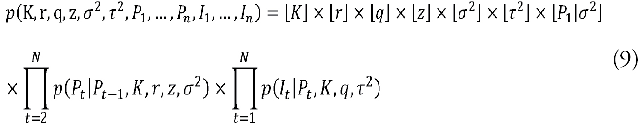
with square brackets indicating densities and N referring to the number of samples. Supplementary information on the above-mentioned general factorisation of Bayesian model (Eq. 9) is available in Wikle et al. 1998 and Clark and Gelfand 2006.

The Markov chain Monte Carlo (MCMC) algorithm using Gibbs sampling was used to explore the joint posterior distributions of the parameters and un-observable states. OpenBugs software (v3.2.3) (Thomas et al. 2006) was used for simulations and was run within R using the R2OpenBugs package (Sturtz et al. 2010). Three chains of 100,000 iterations used to estimate parameters for the model of each fish species. The first 50,000 iterations of each chain were discarded to remove any dependence on initial parameter values; as well, random initial values were generated for each chain. The resulting 50,000 samples were thinned at a rate of 1:5 to remove autocorrelation. This results in a sample size of 10,000 per chain to assess the summary statistics of parameter posterior distributions. Model convergence was assessed with the convergence diagnostics of Geweke (Geweke 1991), Gelman–Rubin’s potential scale reduction measure (Gilks et al. 1996) and Heidelberger and Welch stationarity (Heidelberger and Welch 1983), calculated using the R-package CODA (Plummer et al. 2006).

Table 2 presents the outcomes of three tests for model diagnosis about convergence and stationarity (Plummer et al. 2006).

In the first place, the Geweke diagnostic test was separately applied to verify convergence of the mean of each parameter obtained from the sampled values related to each single chain. In the following, the derived Z-score indicates convergence if its values be less than 2 at absolute value. Thus, as shown in Table 2, for three MCMC chains of all fourteen specified high-commercial demersal fish species, the absolute value of Z-scores is less than 2 which demonstrates that there are no considerable differences in the means of the first and last collections of iterations of the chains. Secondly, the potential scale reduction factor of the Gelman-Rubin diagnostic (Rˆ) is used to investigate the convergence of the chain applying two or more samples produced in parallel. The Rˆ values, approximately close to one, which reveal convergence shows that all MCMC samples of the model parameters reached convergence to posterior distributions. Therefore, according to the results, the Rˆ values are identically one for all the above-mentioned fish species MCMC chains, which are consistent with the convergence in distribution of the MCMC samples to the posterior distributions. The third diagnostic statistic, the Heidelberger-Welch stationarity test, was used to explore the sample convergence of single chains from univariate observations, expressed by p-values. Hence, considering the results, the MCMC chains of all the fish species MCMC simulations passed the Heidelberger and Welch stationarity test, which could not reject the hypothesis that the MCMC chains are stationary at the 95% confidence level for any of the parameters. Generally, the above-described diagnostic convergence tests and visual consideration of trace plots in Appendix 2, confirm that the MCMC chains of all fourteen specified high-commercial demersal fish species produce representative specimens from the joint posterior distribution over the model parameters.

Summary of the posterior descriptive statistics is presented in Table 3, including the posterior means and marginal posteriors with 95% credibility intervals (Crl) (the 2.5% and 97.5% percentiles as lower and upper limits) for Bayesian state-space GSPM parameters of the fourteen specified high-commercial demersal fish species.

Since the intrinsic growth rate r shows the relationship between size and age, it is an important factor in life history theory (Arendt 1997). The marginal posterior means of the intrinsic growth rate (r) for Elutheronema tetradactylum within 95% credibility intervals (0.051, 0.332) indicated that the given available data information (prior distribution) and the true value of (r) falls within (Crl) with 95% probability. Similarly, for all other thirteen fish species, the marginal posterior means of (r) were within 95% credibility intervals of the posterior predictive distributions and it can be concluded that, for the given available data information (prior distribution), the true value of (r) falls within (Crl) 95% probability for them. The posterior means of intrinsic growth rate for Platycephalus indicus and Scomberoides commersonnianus were similar to results attained by Cheung and Sumaila (2015), but for all the other 11 remaining fish species, except for Protonibea diacanthus, the posterior means of intrinsic growth were lower and, for Protonibea diacanthus, it was more than the results of the recently above-mentioned study. The posterior means of all the fish species more than medians indicates that their posterior distributions right skewed. Since the mean and median of posterior distribution of (r) for all fish species was within 95% (Crl), therefore for the given available data information (prior distribution), the true value of (r) falls within (Crl) with 95% probability.

According to the results in Table 3, the marginal posterior means of shape parameter, (z), for Elutheronema tetradactylum was within the 95% credibility intervals (0.112, 2.736), indicating that, for the given available data information (prior distribution), the true value of (z) falls within (Crl) with 95% probability. Similarly, for all other thirteen fish species, the marginal posterior means of (z) were within the 95% credibility intervals of the posterior predictive distributions and it can be concluded that, for the given available data information (prior distribution), the true value of (z) falls within (Crl) with the 95% probability for them. In addition, based on the results, for all Bayesian state-space GSPM, the marginal posterior means for (z), with 95% credible interval, were dissimilar and the posterior means greater than medians indicated that the related posterior distributions were right skewed. The posterior means of shape parameter z for Platycephalus indicus and Scomberoides commersonnianus were more than unity and indicates that the biomass production was increased into peak when the biomass was more than K/2. However, for all the other remaining 12 fish species, the posterior means and medians of shape parameter z were less than unity, indicating that the biomass production peaked when the biomass was less than K/2. As mentioned above and according to the results of Table 3, although the value of the shape parameter z is different from unity for all 14 models, due to the proximity of the value of z with unity, it may be assumed that the classic Schaefer (logistic) surplus production model (SSPM) is a better option than the generalised surplus production model (GSPM). Therefore, the (SSPM) was estimated for all aforesaid fourteen studied fish species and compared with (GSPM) based on predictive performance using the Deviance Information Criterion (DIC), given by Spiegelhalter et al. 2002. In addition, according to Ando (2010), DIC is used to compare the performance of different Bayesian models. It is particularly useful where the posterior distributions of the models have been obtained by MCMC algorithm estimation. Therefore, while comparing different possible models for their similar records, lesser values of DIC recommend better predictive capability. Thus, according to the results of Table 4, the value of DIC for all fish species, based on GSPM, is less than that of SSPM. Therefore, GSPM is more suitable for analysing the present study.

The results of Table 3 identify that the marginal posterior means of carrying capacity, (K), for Elutheronema tetradactylum was within the 95% credibility intervals (621.5, 1975) and indicates that, for the given available data information (prior distribution), the true value of (K) falls within (Crl) with 95% probability. Similarly, for all other thirteen fish species, the marginal posterior means of (K) were within the 95% credibility intervals of the posterior predictive distributions and it can be concluded that, for the given available data information (prior distribution), the true value of (K) falls within (Crl) with 95% probability for them. The posterior means of carrying capacity K with 95% credibility intervals more than the medians as reveals that the posterior distributions right skewed.

The marginal posterior means of the catchability coefficient (q) for Elutheronema tetradactylum was within the 95% credibility intervals (0.0008, 0.002) and indicates that, for the given available data information (prior distribution), the true value of (q) falls within (Crl) with 95% probability. Similarly, for all other thirteen fish species, the marginal posterior means of (q) were within the 95% credibility intervals of the posterior predictive distributions and it can be concluded that for the given available data information (prior distribution), the true value of (q) falls within (Crl) with 95% probability for them. Furthermore, the posterior means and medians of the catchability coefficient (q) with 95% confidence interval for all the studied fish species were equal which shows that their posterior distributions were symmetric.

The marginal posterior means of the process noise variances, (σ²) for Elutheronema tetradactylum was within the 95% credibility intervals (0.004, 0.012) and indicates that, for the given available data information (prior distribution), the true value of (σ²) falls within (Crl) with 95% probability. Similarly, also, for all other thirteen fish species, the marginal posterior means of (σ²) were within the 95% credibility intervals of the posterior predictive distributions and it can be concluded that, for the given available data information (prior distribution), the true value of (σ²) falls within (Crl) with 95% probability for them. In addition, for the process noise variances of Bayesian state-space GSPM of Lutjanus malabaricus, Parastromateus niger, Saurida tumbil and Rhabdosargus sarba with 95% confidence interval, the posterior means were generally higher than the medians because their posterior distributions were right skewed. However, for the other 10 fish species, the posterior means and medians of the process noise variances Ó² were equal which shows that their posterior distributions were symmetric.

The marginal posterior means of the observation noise variances, (τ²) for Elutheronema tetradactylum within 95% credibility intervals (0.206, 0.613), indicates that for the given available data information (prior distribution), the true value of (τ²) falls within (Crl) 95% probability. Similarly, for all other thirteen fish species, the marginal posterior means of (τ²) were within 95% credibility intervals of the posterior predictive distributions and it can be concluded that, for the given available data information (prior distribution), the true value of (τ²) falls within (Crl) with 95% probability for them. In addition, the means and medians marginal posterior of observation noise variances (τ²) of Bayesian state-space GSPM, except for Otolithes ruber, were dissimilar for the other species. For the above-considered fish species, the equality of the posterior mean and median of observation noise variances (τ²) indicates that their posterior distributions were symmetric. However, for all the other remaining 13 fish species, due to the right skewed of their posterior distributions, the means were generally higher than the medians.

A summary of the results of fisheries management reference points derived from Bayesian state-space GSPM is graphically presented for all fourteen specified high-commercial demersal fish species through the stock status plots (i.e. Kobe plots or phase diagrams) in Figure 2; as well, time series of posterior median biomass with confidence intervals is shown in Figure 3.

The Kobe plot characterises, relative biomass (B_S = B / B_MSY) and relative fishing mortality rate (F_S = F / F_MSY) in a graph which provides four different quadrants, each indicating a different population status. The red region is kept for the worst case in which the stock is excessively overfished (B / B_MSY < 1) and, at the same time, the overfishing is at a high rate (F / F_MSY > 1). The green zone denotes a situation where no overfishing is happening (F / F_MSY < 1) and where the stock is not overfished (B / B_MSY > 1), so it is the best condition for the stock. The orange quadrant presents a situation where overfishing is occurring (F / F_MSY > 1), while the stock is not overfished (B / B_MSY > 1), so a decrease in fishing intensity would bring it back to the ideal green condition. The yellow subdivision shows that the stock has been overfished (B / B_MSY < 1), while the overfishing has not occurred (F / F_MSY < 1), so it will recover in due course if the fishing intensity is continued at the existing level.

According to Figure 2, the stock status of Greater lizardfish (Saurida tumbil), Javelin grunter (Pomadasys kaakan) and Tigertooth croaker (Otolithes ruber) are completely (100%) in the red zone. Therefore, these stocks are being excessively overfished and are threatened with extinction. The other situation of fish species, despite being overfished in recent years, is in the yellow subdivision, which indicates that these stocks are not being overfished. So, they will recover in due course if the fishing intensity continues at the existing level. Amongst them, the recovery condition of Bartail flathead (Platycephalus indicus), Fourfinger threadfin (Elutheronema tetradactylum), Malabar blood snapper (Lutjanus malabaricus), Black pomfret (Parastromateus niger) and John’s snapper (Lutjanus johni), is much better due to their high percentage in the yellow zone. Additionally, in terms of recovery condition, the Goldlined seabream (Rhabdosargus sarba), Smalltooth emperors (Lethrinus microdon), Talang queen fish (Scomberoides commersonnianus) and Blackspotted croaker (Protonibea diacanthus) because of their less percentage in the yellow zone are in the second place. Finally, the Silver pomfret (Pampus argenteus) with one percentage in the yellow zone has the worst recovery situation. It can be said that it is located in the red zone and is threatened with extinction. It is noteworthy that the overfishing and overfished results of the described demersal fish species in this research were similar to those previously described (Valinassab et al. 2010; Valinassab et al. 2003; Valinassab et al. 2006; Valinassab et al. 2005). These results about the overfishing and overfished demersal fish species are also similar to those by Osio et al. 2015 who expressed that 95% of the assessed and potentially 98% of the unassessed demersal fish are overexploited. Therefore, regarding the above-described conditions, the fish species extinction may be a possibility in the future.

Simulated biomass time series of the fourteen specified high-commercial demersal fish species with 95% confidence intervals are considerable as shown in Figure 3.

According to the above-described results of the Kobe diagrams, in which all stocks are in critical condition and are threatened with extinction, the trend plots of simulated biomass confirm the previous results, due to the Biomass not having a good increasing trend. As the charts in Figure 3 show, the quantity of Biomass has not improved in recent years for all specified-fish species. If these trends unfortunately continue, the species may be extinct and the livelihoods of fishermen could be lost in the near future.

References

- Ando T (2010) Bayesian model selection and statistical modeling. CRC Press.
- Arendt JD (1997) Adaptive intrinsic growth rates: An integration across taxa. The Quarterly Review of Biology 72(2): 149–177. https://doi.org/10.1086/419764
- Berkes F (2001) Managing small-scale fisheries: alternative directions and methods. IDRC.
- Berliner LM (1996) Hierarchical Bayesian time series models. Maximum entropy and Bayesian methods. Springer, 15-22.
- Bishop J (2006) Standardizing fishery-dependent catch and effort data in complex fisheries with technology change. Reviews in Fish Biology and Fisheries 16(1): 21–38. https://doi.org/10.1007/s11160-006-0004-9
- Brodziak J, Ishimura G (2011) Development of Bayesian production models for assessing the North Pacific swordfish population. Fisheries Science 77(1): 23–34. https://doi.org/10.1007/s12562-010-0300-0
- Buckland S, Newman K, Thomas L, Koesters N (2004) State-space models for the dynamics of wild animal populations. Ecological Modelling 171(1-2): 157–175. https://doi.org/10.1016/j.ecolmodel.2003.08.002
- Chaloupka M, Balazs G (2007) Using Bayesian state-space modelling to assess the recovery and harvest potential of the Hawaiian green sea turtle stock. Ecological Modelling 205(1-2): 93–109. https://doi.org/10.1016/j.ecolmodel.2007.02.010
- Chen Y, Chen L, Stergiou KI (2003) Impacts of data quantity on fisheries stock assessment. Aquatic Sciences 65(1): 92–98. https://doi.org/10.1007/s000270300008
- Cheung WW, Sumaila UR (2015) Economic incentives and overfishing: A bioeconomic vulnerability index. Marine Ecology Progress Series 530: 223–232. https://doi.org/10.3354/meps11135
- Clark JS, Gelfand AE (2006) Hierarchical modelling for the environmental sciences: statistical methods and applications. Oxford University Press on Demand.
- Costello C, Ovando D, Hilborn R, Gaines SD, Deschenes O, Lester SE (2012) Status and solutions for the world’s unassessed fisheries. Science 338(6106): 517–520. https://doi.org/10.1126/science.1223389
- De Valpine P, Hastings A (2002) Fitting population models incorporating process noise and observation error. Ecological Monographs 72(1): 57–76. https://doi.org/10.1890/0012-9615(2002)072[0057:FPMIPN]2.0.CO;2
- Fletcher R (1978) On the restructuring of the Pella-Tomlinson system. Fish Bulletin 76: 515–521.
- Gelman A, Carlin JB, Stern HS, Rubin DB (2014) Bayesian data analysis. Chapman & Hall/CRC Boca Raton, FL, USA.
- Gelman A, Meng X-L (2004) Applied Bayesian modeling and causal inference from incomplete-data perspectives. John Wiley & Sons.
- Geweke J (1991) Evaluating the accuracy of sampling-based approaches to the calculation of posterior moments. Federal Reserve Bank of Minneapolis, Research Department Minneapolis, MN, USA.
- Gilks WR, Richardson S, Spiegelhalter DJ (1996) Introducing markov chain monte carlo. Markov chain Monte Carlo in practice 1: 19.
- Haddon M (2010) Modelling and quantitative methods in fisheries. CRC press.
- Harley SJ, Myers RA, Dunn A (2001) Is catch-per-unit-effort proportional to abundance? Canadian Journal of Fisheries and Aquatic Sciences 58(9): 1760–1772. https://doi.org/10.1139/f01-112
- Heidelberger P, Welch PD (1983) Simulation run length control in the presence of an initial transient. Operations Research 31(6): 1109–1144. https://doi.org/10.1287/opre.31.6.1109
- Hilborn R, Walters CJ (1992) Quantitative fisheries stock assessment: Choice, dynamics and uncertainty. Reviews in Fish Biology and Fisheries 2(2): 177–178. https://doi.org/10.1007/BF00042883
- Jiao Y, Cortés E, Andrews K, Guo F (2011) Poor‐data and data‐poor species stock assessment using a Bayesian hierarchical approach. Ecological Applications 21(7): 2691–2708. https://doi.org/10.1890/10-0526.1
- Jiao Y, Neves R, Jones J (2008) Models and model selection uncertainty in estimating growth rates of endangered freshwater mussel populations. Canadian Journal of Fisheries and Aquatic Sciences 65(11): 2389–2398. https://doi.org/10.1139/F08-141
- Kéry M, Schaub M (2011) Bayesian population analysis using WinBUGS: a hierarchical perspective. Academic Press.
- Kinas PG (1996) Bayesian fishery stock assessment and decision making using adaptive importance sampling. Canadian Journal of Fisheries and Aquatic Sciences 53(2): 414–423. https://doi.org/10.1139/f95-189
- King R, Morgan B, Gimenez O, Brooks S (2009) Bayesian analysis for population ecology. CRC Press.
- Kuparinen A, Mäntyniemi S, Hutchings JA, Kuikka S (2012) Increasing biological realism of fisheries stock assessment: Towards hierarchical Bayesian methods. Environmental Reviews 20(2): 135–151. https://doi.org/10.1139/a2012-006
- Laloë F (1995) Should surplus production models be fishery description tools rather than biological models? Aquatic Living Resources 8(1): 1–16. https://doi.org/10.1051/alr:1995001
- Mäntyniemi SHP, Whitlock RE, Perälä TA, Blomstedt PA, Vanhatalo JP, Rincón MM, Kuparinen AK, Pulkkinen HP, Kuikka OS (2015) General state-space population dynamics model for Bayesian stock assessment. ICES Journal of Marine Science: Journal du Conseil 72(8): 2209–2222. https://doi.org/10.1093/icesjms/fsv117
- Matthew S (2003) Small-scale fisheries perspectives on an ecosystem-based approach to fisheries management. Responsible Fisheries in the Marine Ecosystem, FAO, Rome: 47–64.
- McAllister MK, Kirkwood G (1998) Using Bayesian decision analysis to help achieve a precautionary approach for managing developing fisheries. Canadian Journal of Fisheries and Aquatic Sciences 55(12): 2642–2661. https://doi.org/10.1139/f98-121
- Meyer R, Millar RB (1999) BUGS in Bayesian stock assessments. Canadian Journal of Fisheries and Aquatic Sciences 56(6): 1078–1087. https://doi.org/10.1139/f99-043
- Millar RB (2002) Reference priors for Bayesian fisheries models. Canadian Journal of Fisheries and Aquatic Sciences 59(9): 1492–1502. https://doi.org/10.1139/f02-108
- Montenegro C, Branco M (2016) Bayesian state-space approach to biomass dynamic models with skewed and heavy-tailed error distributions. Fisheries Research 181: 48–62. https://doi.org/10.1016/j.fishres.2016.03.021
- Neiland AE, Béné C (2013) Poverty and small-scale fisheries in West Africa. Springer Science & Business Media.
- Osio GC, Orio A, Millar CP (2015) Assessing the vulnerability of Mediterranean demersal stocks and predicting exploitation status of un-assessed stocks. Fisheries Research 171: 110–121. https://doi.org/10.1016/j.fishres.2015.02.005
- Pakzad HR, Pasandi M, Soleimani M, Kamali M (2014) Distribution and origin of heavy metals in the sand sediments in a sector of the Oman Sea (the Sistan and Baluchestan province, Iran). Quaternary International 345: 138–147. https://doi.org/10.1016/j.quaint.2014.03.031
- Parent E, Rivot E (2012) Introduction to hierarchical Bayesian modeling for ecological data. CRC Press.
- Pauly D (2006) Major trends in small-scale marine fisheries, with emphasis on developing countries, and some implications for the social sciences. Maritime Studies 4: 7–22.
- Pella JJ, Tomlinson PK (1969) A generalized stock production model. Inter-American Tropical Tuna Commission.
- Plummer M, Best N, Cowles K, Vines K (2006) CODA: Convergence diagnosis and output analysis for MCMC. R News 6: 7–11.
- Punt AE, Hilborn RAY (1997) Fisheries stock assessment and decision analysis: The Bayesian approach. Reviews in Fish Biology and Fisheries 7(1): 35–63. https://doi.org/10.1023/A:1018419207494
- Punt AE, Smith DC, Smith ADM (2011) Among-stock comparisons for improving stock assessments of data-poor stocks: The “Robin Hood” approach. ICES Journal of Marine Science: Journal du Conseil 68(5): 972–981. https://doi.org/10.1093/icesjms/fsr039
- Punt AE, Szuwalski C (2012) How well can F MSY and B MSY be estimated using empirical measures of surplus production? Fisheries Research 134: 113–124. https://doi.org/10.1016/j.fishres.2012.08.014
- Quinn TJ, Deriso RB (1999) Quantitative fish dynamics. Oxford University Press.
- Rankin PS, Lemos RT (2015) An alternative surplus production model. Ecological Modelling 313: 109–126. https://doi.org/10.1016/j.ecolmodel.2015.06.024
- Salas S, Chuenpagdee R, Seijo JC, Charles A (2007) Challenges in the assessment and management of small-scale fisheries in Latin America and the Caribbean. Fisheries Research 87(1): 5–16. https://doi.org/10.1016/j.fishres.2007.06.015
- Schaefer MB (1957) A study of the dynamics of the fishery for yellowfin tuna in the eastern tropical Pacific Ocean. Inter-American Tropical Tuna Commission.
- Seaman JW III, Seaman Jr JW, Stamey JD (2012) Hidden Dangers of Specifying Noninformative Priors. The American Statistician 66(2): 77–84. https://doi.org/10.1080/00031305.2012.695938
- Spiegelhalter DJ, Best NG, Carlin BP, Van Der Linde A (2002) Bayesian measures of model complexity and fit. Journal of the Royal Statistical Society. Series B, Statistical Methodology 64(4): 583–639. https://doi.org/10.1111/1467-9868.00353
- Sturtz S, Ligges U, Gelman A (2010) R2OpenBUGS: a package for running OpenBUGS from R. http://wwwcranrprojectorg/web/packages/R2OpenBUGS/vignettes/R2OpenBUGSpdf
- Thomas A, O’Hara B, Ligges U, Sturtz S (2006) Making BUGS open. R News 6: 12–17.
- Valinassab T, Adjeer M, Momeni M (2010) Biomass estimation of demersal fishes in the Persian Gulf and Oman Sea by swept area method. Final Report. Iranian Fisheries Research Organization Press, Tehran.
- Valinassab T, Daryanabard R, Dehghani R (2003) Monitoring of demersal resources by swept area method in the Oman Sea waters. Final Report. Tehran, Iran
- Valinassab T, Daryanabard R, Dehghani R, Pierce GJ (2006) Abundance of demersal fish resources in the Persian Gulf and Oman Sea. Journal of the Marine Biological Association of the United Kingdom 86(06): 1455–1462. https://doi.org/10.1017/S0025315406014512
- Valinassab T, Dehghani R, Khorshidian K (2005) Biomass estimation of demersal resources in the Persian Gulf and Gulf of Oman by swept area method. Final Report Iranian Fisheries Research Organization (IFRO), Tehran, 121 pp.
- Wikle CK, Berliner LM, Cressie N (1998) Hierarchical Bayesian space-time models. Environmental and Ecological Statistics 5(2): 117–154. https://doi.org/10.1023/A:1009662704779
- Xiao Y (1998) Two simple approaches to use of production models in fish stock assessment. Fisheries Research 34(1): 77–86. https://doi.org/10.1016/S0165-7836(97)00064-7
- Ye Y, Dennis D (2009) How reliable are the abundance indices derived from commercial catch-effort standardization? Canadian Journal of Fisheries and Aquatic Sciences 66(7): 1169–1178. https://doi.org/10.1139/F09-070
- Yu H, Jiao Y, Carstensen LW (2013) Performance comparison between spatial interpolation and GLM/GAM in estimating relative abundance indices through a simulation study. Fisheries Research 147: 186–195. https://doi.org/10.1016/j.fishres.2013.06.002
- Zhu X, Day AC, Carmichael TJ, Tallman RF (2014) Hierarchical Bayesian Modeling for Cambridge Bay Arctic Char, Salvelinus Alpinus (L.), Incorporated with Precautionary Reference Points.
Appendix 1
Procedure of prior distributions functions used for parameters of all Bayesian state-space GSPM
Log-normal distribution procedure for intrinsic growth rate (r)
Standard Deviation = x
Average of Intrinsic Growth Rate (r) = y
Precision of Prior = 1/log(1 + x^2)
Average of Prior = log(y) – (0.5/ Precision of Prior)
r ~ dlnorm (Average of prior, Precision of prior)
Inverse Gamma Distribution Procedure for the Process and Observation Noise Variances
Shape Parameter = x
Scale Parameter=y
Gamma ~ dgamma (x, y)
Inverse-Gamma = 1/Gamma
Log-Normal Distribution Procedure for Initial Relative Biomass P[1]
B0=the Biomass in First Time
Kmin=minimum carrying capacity is considered equal to minimum Historical catches.
Kmax= maximum carrying capacity is considered equal to ten times the minimum Historical catches.
Pi ~ dunif(B0/Kmax, B0/Kmin)
isigma= Inverse Gamma Distribution for process noise variances
Pm[1] <- log(Pi)
P[1] ~ dlnorm(Pm[1], isigma)
Appendix 2
Trace plots for Bayesian state-space GSPM parameters (r, K, q, z, (sigma), and (tau)) for fourteen studied demersal fish species. Consider figures A1–14.